In optimizing compilers, data structure choices directly influence the power and efficiency of practical program optimization. A poor choice of data structure can inhibit optimization or slow compilation to the point that advanced optimization features become undesirable. Recently, static single assignment form and the control dependence graph have been proposed to represent data flow and control flow properties of programs. Each of these previously unrelated techniques lends efficiency and power to a useful class of program optimizations. Although both of these structures are attractive, the difficulty of their construction and their potential size have discouraged their use. We present new algorithms that efficiently compute these data structures for arbitrary control flow graphs. The algorithms use dominance frontiers, a new concept that may have other applications. We also give analytical and experimental evidence that all of these data structures are usually linear in the size of the original program. This paper thus presents strong evidence that these structures can be of practical use in optimization.
Categories and Subject Descriptors: D.3.3 [Programming Languages]: Language Constructs—control structures; data types and structures; procedures, functions and subroutines; D.3.4 [Programming Languages]: Processors—compilers; optimization; I.1.2 [Algebraic Manipulation]: Algorithms—analysis of algorithms; I.2.2 [Artificial Intelligence]: Automatic Programming—program transformation
A preliminary version of this paper, “An Efficient Method of Computing Static Single Assignment Form,” appeared in the Conference Record of the 16th ACM Symposium on Principles of Programming Languages (Jan. 1989). F. K. Zadeck’s work on this paper was partially supported by the IBM Corporation, the Office of Naval Research, and the Defense Advanced Research Projects Agency under contract N00014-83-K-0146 and ARPA order 6320, Amendment 1. Authors’ addresses: R. Cytron, J. Ferrante, and M. N. Wegman, Computer Sciences Department, IBM Research Division, P. O. Box 704, Yorktown Heights, NY 10598; B. K. Rosen, Mathematical Sciences Department, IBM Research Division, P. O. Box 218, Yorktown Heights, NY 10598; F. K. Zadeck, Computer Science Department, P.O. Box 1910, Brown University, Providence, RI 02912. Permission to copy without fee all or part of this material is granted provided that the copies are not made or distributed for direct commercial advantage, the ACM copyright notice and the title of the publication and its date appear, and notice is given that copying is by permission of the Association for Computing Machinery. To copy otherwise, or to republish, requires a fee and/or specific permission. © 1991 ACM 0164-0925/91/1000-0451 \$01.50
General Terms: Algorithms, Languages Additional Key Words and Phrases: Control dependence, control flow graph, def-use chain, dominator, optimizing compilers
1 INTRODUCTION
In optimizing compilers, data structure choices directly influence the power and efficiency of practical program optimization. A poor choice of data structure can inhibit optimization or slow compilation to the point where advanced optimization features become undesirable. Recently, static single assignment (SSA) form [5, 43] and the control dependence graph [24] have been proposed to represent data flow and control flow properties of programs. Each of these previously unrelated techniques lends efficiency and power to a useful class of program optimizations. Although both of these structures are attractive, the difficulty of their construction and their potential size have discouraged their use [4]. We present new algorithms that efficiently compute these data structures for arbitrary control flow graphs. The algorithms use dominance frontiers, a new concept that may have other applications. We also give analytical and experimental evidence that the sum of the sizes of all the dominance frontiers is usually linear in the size of the original program. This paper thus presents strong evidence that SSA form and control dependences can be of practical use in optimization.
Figure 1 illustrates the role of SSA form in a compiler. The intermediate code is put into SSA form, optimized in various ways, and then translated back out of SSA form. Optimizations that can benefit from using SSA form include code motion [22] and elimination of partial redundancies [43], as well as the constant propagation discussed later in this section.
Variants of SSA form have been used for detecting program equivalence [5, 52] and for increasing parallelism in imperative programs [21]. The representation of simple data flow information (def-use chains) may be made more compact through SSA form. If a variable has definitions and uses, then there can be def-use chains. When similar information is encoded in SSA form, there can be at most def-use chains, where is the number of edges in the control flow graph [40]. Moreover, the def-use information encoded in SSA form can be updated easily when optimizations are applied. This is important for a constant propagation algorithm that deletes branches to code proven at compile time to be unexecutable [50]. Specifically, the def-use information is just a list, for each variable, of the places in the program text that use that variable. Every use of V is indeed a use of the value provided by the (unique) assignment to V.
To see the intuition behind SSA form, it is helpful to begin with straight-line code. Each assignment to a variable is given a unique name (shown as a subscript in Figure 2), and all of the uses reached by that assignment are renamed to match the assignment’s new name.
Most programs, however, have branch and join nodes. At the join nodes, we add a special form of assignment called a -function. In Figure 3, the
Original Intermediate Code ↓ Optimized Intermediate Code ↑
Fig. 1. Vertical arrows represent translation to/from static single assignment form. Horizontal arrows represent optimizations.

              if P
then V ← 4
else V ← 6
/ Use V several times. /
              if P
then V₁ ← 4
else V₂ ← 6
/ Use V_3 several times. /

operands to the -function indicate which assignments to reach the join point. Subsequent uses of become uses of . The old variable is thus replaced by new variables , and each use of is reached by just one assignment to . Indeed, there is only one assignment to in the entire program. This simplifies the record keeping for several optimizations. An especially clear example is constant propagation based on SSA form [50]; the next subsection sketches this application.
1.1 Constant Propagation
Figure 4 is a more elaborate version of Figure 3. The else branch includes a test of , and propagating the constant true to this use of tells a compiler that the else branch never falls through to the join point. If is the constant true, then all uses of after the join point are really uses of the constant 4. Such possibilities can be taken into account without SSA form, but the processing is either costly [48] or difficult to understand [49]. With SSA form, the algorithm is fast and simple.
Initially, the algorithm assumes that each edge is unexecutable (i.e., never followed at run time) and that each variable is constant with an as-yet unknown value (denoted ). Worklists are initialized appropriately, and the assumptions are corrected until they stabilize. Suppose the algorithm finds that variable is not constant (denoted ) and, hence, that either branch of
              if P
then do V ← 4
    end
else do V ← 6
    if Q then return
end
... ← V + 5
              if P
then do V₁ ← 4
    end
else do V₂ ← 6
    if Q then return
end
V₃ ← φ(V₁, V₂)
... ← V₃ + 5
Fig 4. Example of constant propagation.
the outer conditional may be taken. The outedges of the test of P are marked executable, and the statements they reach are processed. When V₁ ← 4 is processed, the assumption about V₁ is changed from T to 4, and all uses of V₁ are notified that they are uses of 4. (Each use of V₁ is indeed a use of this value, thanks to the single assignment property.) In particular, the φ-function combines 4 with V₂. The second operand of the φ-function, however, is associated with the inedge of the join point that corresponds to falling through the else branch. So long as this edge is considered unexecutable, the algorithm uses T for the second operand, no matter what is currently assumed about V₂. Combining 4 with T yields 4, so uses of V₃ are still tentatively assumed to be uses of 4. Eventually, the assumption about Q may change from T to a known constant or to ⊥. A change to either false or ⊥ would lead to the discovery that the second inedge of the join point can be followed, and then the 6 at V₂ combines with the 4 at V₁ to yield ⊥ at V₃. A change to true would have no effect on the assumption at V₃. Traditional constant propagation algorithms, on the other hand, would see that assignments of two different constants to V seem to “reach” all uses after the join point. They would thus decide that V is not constant at these uses.
The algorithm just sketched is linear in the size of the SSA program it sees [50], but this size might be nonlinear in the size of the original program. In particular, it would be safe but inefficient to place a φ-function for every variable at every join point. This paper shows how to obtain SSA form efficiently. When φ-functions are placed carefully, nonlinear behavior is still possible but is unlikely in practice. The size of the SSA program is typically linear in the size of the original program; the time to do the work is essentially linear in the SSA size.
1.2 Where to Place φ-Functions
At first glance, careful placement might seem to require the enumeration of pairs of assignment statements for each variable. Checking whether there are two assignments to V that reach a common point might seem to be intrinsically nonlinear. In fact, however, it is enough to look at the dominance frontier of each node in the control flow graph. Leaving the technicalities to later sections, we sketch the method here.
Suppose that a variable V has just one assignment in the original program, so that any use of V will be either a use of the value V₀ at entry to the program or a use of the value V₁ from the most recent execution of the assignment to V. Let X be the basic block of code that assigns to V, so X will determine the value of V when control flows along any edge X → Y to a basic block Y. When entered along X → Y, the code in Y will see V₁ and be unaffected by V₀. If Y ≠ X, but all paths to Y must still go through X (in which case X is said to strictly dominate Y), then the code in Y will always see V₁. Indeed, any node strictly dominated by X will always see V₁, no matter how far from X it may be. Eventually, however, control may be able to reach a node Z not strictly dominated by X. Suppose Z is the first such node on a path, so that Z sees V₁ along one inedge but may see V₀ along another inedge. Then Z is said to be in the dominance frontier of X and is clearly in need of a φ-function for V. In general, no matter how many assignments to V may appear in the original program and no matter how complex the control flow may be, we can place φ-functions for V by finding the dominance frontier of every node that assigns to V, then the dominance frontier of every node where a φ-function has already been placed, and so on.
The same concept of dominance frontiers used for computing SSA form can also be used to compute control dependences [20, 24], which identify those conditions affecting statement execution. Informally, a statement is control dependent on a branch if one edge from the branch definitely causes that statement to execute while another edge can cause the statement to be skipped. Such information is vital for detection of parallelism [2], program optimization, and program analysis [28].
1.3 Outline of the Rest of the Paper
Section 2 reviews the representation of control flow by a directed graph. Section 3 explains SSA form and sketches how to construct it. This section also considers variants of SSA form as defined here. Our algorithm can be adjusted to deal with these variants. Section 4 reviews the dominator tree concept and formalizes dominance frontiers. Then we show how to compute SSA form (Section 5) and the control dependence graph (Section 6) efficiently. Section 7 explains how to translate out of SSA form. Section 8 shows that our algorithms are linear in the size of programs restricted to certain control structures. We also give evidence of general linear behavior by reporting on experiments with FORTRAN programs. Section 9 summarizes the algorithms and time bounds, compares our technique with other techniques, and presents some conclusions.
2 CONTROL FLOW GRAPHS
The statements of a program are organized into (not necessarily maximal) basic blocks, where program flow enters a basic block at its first statement and leaves the basic block at its last statement [1, 36]. Basic blocks are indicated by the column of numbers in parentheses in Figure 5. A control flow graph is a directed graph whose nodes are the basic blocks of a program and two additional nodes, Entry and Exit. There is an edge from Entry to
              I ← 1	(1)
J ← 1	(1)
K ← 1	(1)
L ← 1	(1)
repeat	(2)
    if (P)	(2)
        then do	(3)
            J ← I	(3)
            if (Q)	(3)
                then L ← 2	(4)
                else L ← 3	(5)
            K ← K + 1	(6)
        end	(6)
    else K ← K + 2	(7)
print(I,J,K,L)	(8)
repeat	(9)
    if (R)	(9)
        then L ← L + 4	(10)
until (S)	(11)
I ← I + 6	(12)
until (T)	(12)
Fig 5 Simple program and its control flow graph.
any basic block at which the program can be entered, and there is an edge to Exit from any basic block that can exit the program. For reasons related to the representation of control dependences and explained in Section 6, there is also an edge from Entry to Exit. The other edges of the graph represent transfers of control (jumps) between the basic blocks. We assume that each node is on a path from Entry and on a path to Exit. For each node X, a successor of X is any node Y with an edge X → Y in the graph, and Succ(X) is the set of all successors of X; similarly for predecessors. A node with more than one successor is a branch node; a node with more than one predecessor is a join node. Finally, each variable is considered to have an assignment in Entry to represent whatever value the variable may have when the program is entered. This assignment is treated just like the ones that appear explicitly in the code. Throughout this paper, CFG denotes the control flow graph of the program under discussion.
For any nonnegative integer J, a path of length J in CFG consists of a sequence of J + 1 nodes (denoted X₀, ..., X_J) and a sequence of J edges (denoted e₁, ..., e_J) such that e_j runs from X_{j-1} to X_j for all j with 1 ≤ j ≤ J. (We write e_j: X_{j-1} → X_j.) As is usual with sequences, one item (node or edge) may occur several times. The null path, with J = 0, is allowed. We write for an unrestricted path , but if is known to be nonnull.
Nonnull paths and are said to converge at a node if
Intuitively, the paths and start at different nodes and are almost node-disjoint, but they come together at the end. The use of or rather than and in (3) is deliberate. One of the paths may happen to be a cycle , but we still need to consider the possibility of convergence.
3 STATIC SINGLE ASSIGNMENT FORM
This section initially assumes that programs have been expanded to an intermediate form in which each statement evaluates some expressions and uses the results either to determine a branch or to assign to some variables. (Other program constructs are considered in Section 3.1.) An assignment statement has the form , where the left-hand side is a tuple of distinct target variables and the right-hand side is a tuple of expressions, with the same length as the tuple. Each target variable in is assigned the corresponding value from . In the examples already discussed, all tuples are 1-tuples, and there is no need to distinguish between and . Section 3.1 sketches the use of longer tuples in expanding other program constructs (such as procedure calls) so as to make explicit the variables used and/or changed by the statements in the source program. Such explicitness is a prerequisite for most optimizations anyway. The only novelty in our use of tuples is the fact that they provide a simple and uniform way to fold the results of analysis into the intermediate text. Practical concerns about the size of the intermediate text are addressed in Section 3.1.
Translating a program into SSA form is a two-step process. In the first step, some trivial -functions are inserted at some of the join nodes in the program's control flow graph. In the second step, new variables (for ) are generated. Each mention of a variable in the program is replaced by a mention of one of the new variables , where a mention may be in a branch expression or on either side of an assignment statement. Throughout this paper, an assignment statement may be either an ordinary assignment or a -function. Figure 6 displays the result of translating a simple program to SSA form.
A -function at entrance to a node has the form , where are variables. The number of operands is the number of control flow predecessors of . The predecessors of are listed in some arbitrary fixed order, and the th operand of is associated with the th
              I ← 1
J ← 1
K ← 1
L ← 1
repeat
    I₁ ← 1
    J₁ ← 1
    K₁ ← 1
    L₁ ← 1
    repeat
        I₂ ← φ(I₃, I₁)
        J₂ ← φ(J₄, J₁)
        K₂ ← φ(K₅, K₁)
        L₂ ← φ(L₉, L₁)
        if (P)
            then do
                J ← I
                if (Q)
                    then L ← 2
                    else L ← 3
                K ← K + 1
            end
        else K ← K + 2
    print(I, J, K, L)
    repeat
        if (R)
            then L ← L + 4
        until (S)
        I ← I + 6
until (T)

I₁ ← 1
J₁ ← 1
K₁ ← 1
L₁ ← 1
repeat
    I₂ ← φ(I₃, I₁)
    J₂ ← φ(J₄, J₁)
    K₂ ← φ(K₅, K₁)
    L₂ ← φ(L₉, L₁)
    if (P)
        then do
            J₃ ← I₂
            if (Q)
                then L₃ ← 2
                else L₄ ← 3
            L₅ ← φ(L₃, L₄)
            K₃ ← K₂ + 1
        end
    else K₄ ← K₂ + 2
        J₄ ← φ(J₃, J₂)
        K₅ ← φ(K₃, K₄)
        L₆ ← φ(L₂, L₅)
    print(I₂, J₄, K₅, L₆)
    repeat
        L₇ ← φ(L₉, L₆)
        if (R)
            then L₈ ← L₇ + 4
            L₉ ← φ(L₈, L₇)
        until (S)
        I₃ ← I₂ + 6
    until (T)
Fig. 6 Simple program and its SSA form.
predecessor. If control reaches X from its jth predecessor, then the run-time support¹ remembers j while executing the φ-functions in X. The value of φ(R, S, ...) is just the value of the jth operand. Each execution of a φ-function uses only one of the operands, but which one depends on the flow of control just before entering X. Any φ-functions in X are executed before the ordinary statements in X. Some variants of φ-functions as defined here are useful for special purposes. For example, each φ-function can be tagged
¹When SSA form is used only as an intermediate form (Figure 1), there is no need actually to provide this support. For us, the semantics of φ are only important when assessing the correctness of intermediate steps in a sequence of program transformations beginning and ending with code that has no φ-functions. Others [6, 11, 52] have found it useful to give φ another parameter that incidentally encodes j, under various restrictions on the control flow.
with the node where it appears [5]. When the control flow of a language is suitably restricted, each -function can be tagged with information about conditionals or loops [5, 6, 11, 52]. The algorithms in this paper apply to such variants as well.
SSA form may be considered as a property of a single program or as a relation between two programs. A single program is defined to be in SSA form if each variable is a target of exactly one assignment statement in the program text. Translation to SSA form replaces the original program by a new program with the same control flow graph. For every original variable , the following conditions are required of the new program:
(1) If two nonnull paths and converge at a node , and nodes and contain assignments to (in the original program), then a trivial -function has been inserted at (in the new program). (2) Each mention of in the original program or in an inserted -function has been replaced by a mention of a new variable , leaving the new program in SSA form. (3) Along any control flow path, consider any use of a variable (in the original program) and the corresponding use of (in the new program). Then and have the same value.
Translation to minimal SSA form is translation to SSA form with the proviso that the number of -functions inserted is as small as possible, subject to Condition (1) above. The optimizations that depend on SSA form are still valid if there are some extraneous -functions beyond those that would appear in minimal SSA form. However, extraneous -functions can cause information to be lost, and they always add unnecessary overhead to the optimization process itself. Thus, it is important to place -functions only where they are required. One variant of SSA form [52] would sometimes forego placing a -function at a convergence point , so long as there are no more uses for in or after . The -function could then be omitted without any risk of losing Condition (3). This has been called pruned SSA form [16], and it is sometimes preferable to our placement at all convergence points. However, as Figure 16 in Section 7 illustrates, our form is sometimes preferable to pruned form. When desired, pruned SSA form can be obtained by a simple adjustment of our algorithm [16, Section 5.1].
For any variable , the nodes at which we should insert -functions in the original program can be defined recursively by Condition (1) in the definition of SSA form. A node needs a -function for if is a convergence point for two paths that originate at two different nodes, both nodes containing assignments to or needing -functions for . Nonrecursively, we may observe that a node needs a -function for because is a convergence point for two nonnull paths and that start at nodes and already containing assignments to . If did not already contain an assignment to , then the -function inserted at adds to the set of nodes that contain assignments to . With more nodes to consider as origins of paths, we may observe more nodes appearing as convergence points of nonnull paths originating at nodes with assignments to V. The set of nodes needing -functions could thus be found by iterating an observation/insertion cycle. The algorithm presented here obtains the same end results in much less time.
3.1 Other Program Constructs
If the source program computes expressions using constants and scalar variables to assign values to scalar variables, then it is straightforward to derive an intermediate text that is ready to be put into SSA form (or otherwise analyzed and transformed by an optimizing compiler). However, source programs commonly use other constructs as well: Some variables are not scalars, and some computations do not explicitly indicate which variables they use or change. This section sketches how to map some important constructs to an explicit intermediate text suitable for use in a compiler.
3.1.1 Arrays. It will suffice to consider one-dimensional arrays here. Arrays of higher dimension involve more notation but no more concerns.
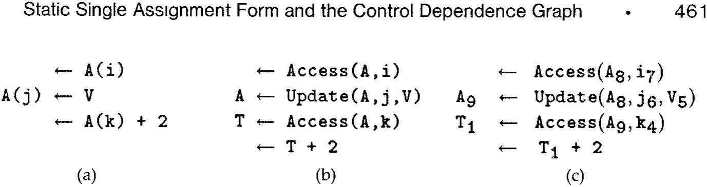
If A and B are array variables, then array assignment statements like A \leftarrow B or A \leftarrow 0, if allowed by the source language, can be treated just like assignments to scalar variables. Many of the mentions of A(i) for some index i, which may be taken to be an integer variable. Treating A(i) as a variable would be awkward, both because an assignment to A(i) may or may not change the value of A(j) and because the value of A(i) could be changed by assigning to i rather than to A(i). An easier approach is illustrated in Figure 7. The entire array is treated like a single scalar variable, which may be one of the operands of Access or Update. The expression Access(A, i) evaluates to the ith component of A; the expression Update(A, j, V) evaluates to an array value that is of the same size as A and has the same component values, except for V as the value of the jth component. Assigning a scalar value V to A(j) is equivalent to assigning an array value to the entire array A, where the new array value depends on the old one, as well as on the index j and on the new scalar value V. The translation to SSA form is unconcerned with whether the values of variables are large objects or what the operators mean.
As with scalars, translation of array references to SSA form removes some anti- and output-dependences [32]. In the program in Figure 7a, dependence analysis may prohibit reordering the use of A(i) by the first statement and the definition of A(j) by the second statement. After translation to SSA form, the two references to A have been renamed, and reordering is then possible. For example, the two statements can execute concurrently. Where optimization does not reorder the two references, Section 7.2 describes how translation out of SSA form reclaims storage that would otherwise be necessary to maintain distinct variables.
\footnotetext{ In typical cases, paths originating at -functions add nothing beyond the contributions from paths originating at ordinary assignments. The straightforward iteration is still too slow, even in typical cases This notation is similar to Select and Update [24], which, in turn, is similar to notation for referencing aggregate structures in a data flow language [23]. }
(a) (b) (c)
Consider the loop shown in Figure 8a, which assigns to every component of array A. The value assigned to each component does not depend (even indirectly) on any of the values previously assigned to components of A. In terms of its effect on A, the whole loop is like an assignment of the form , where A is not used in (\ldots). Any assignment to a component of A that is not used before entering such an initialization loop is dead code that should be eliminated. With or without SSA form, the Update operator in Figure 8b makes A appear to be live at entry to the loop.
One reasonable response to the crudeness of the Update operator is to accept it. Address calculations and other genuine scalar calculations can still be optimized extensively. Another response is to perform dependence analysis [3, 10, 32, 51], which can sometimes determine that no subsequent accesses of A require values produced by any other assignment to A. Such is the case for each execution of the assignment to in Figure 8a. The assignment statement can then be viewed as an initialization of A. The problem for us, or for anyone who uses Update to make arrays look like scalars, is to communicate some of the results of dependence analysis to optimizations (like dead code elimination) that are usually formulated in terms of "scalar" variables. A simple solution to this formal problem is shown in Figure 8c, where the HiddenUpdate operator does not mention the assigned array operand. The actual code generated for an assignment from a HiddenUpdate expression is exactly the same as for an assignment from the corresponding Update expression, where the hidden operand is supplied by the target of the assignment.
3.1.2 Structures. A structure can be generally regarded as an array, where references to structure fields are treated as references to elements of the array. Thus, an assignment to a structure field is translated into an Update of the structure, and a use of a structure field is translated into an Access of the structure. In the prevalent case of simple structure field references, this treatment results in arrays whose elements are indexed by constants. Dependence analysis can often determine independence among such accesses, so that optimizations may move an assignment to one field far from an assignment to another field. If analysis or language semantics reveals a structure whose n fields are always accessed disjointly, then the structure can be decomposed into distinct variables. The elements of such structures are united in the source program only for organizational reasons, and the expression of the structure's decomposition in SSA form makes the program's actual use of the structure more apparent to subsequent optimization.
              integer A(1:100)
integer A₀(1:100)
integer A₁(1:100)
integer A₂(1:100)
i ← 1
repeat
    i₂ ← φ(i₁, i₃)
    A₁ ← φ(A₀, A₂)
    A₂ ← Update(A₁, i₂, i₂)
    i₃ ← i₂ + 1
    A(i) ← i
    i ← i + 1
until i ≥ 100
              (a)
integer A_0(1:100)
integer A_1(1:100)
integer A_2(1:100)
i_1 ← 1
repeat
    i_2 ← φ(i_1, i_3)
    A_1 ← φ(A_0, A_2)
    A_2 ← HiddenUpdate(i_2, i_2)
    i_3 ← i_2 + 1
until i_3 ≥ 100

(b)
integer A_0(1:100)
integer A_1(1:100)
integer A_2(1:100)
i_1 ← 1
repeat
    i_2 ← φ(i_1, i_3)
    A_1 ← φ(A_0, A_2)
    A_2 ← HiddenUpdate(i_2, i_2)
    i_3 ← i_2 + 1
until i_3 ≥ 100
(c)
Fig. 8. Source loop with array assignment (a) is equivalent to code with an Update operator that treats the array A just like a scalar (b). As Section 7.2 explains, the eventual translation out of SSA form will leave just one array here. Using HiddenUpdate (c) is a purely formal way to summarize some results of dependency analysis, if available.
3.1.3 Implicit References to Variables. The construction of SSA form requires knowing those variables modified and used by a statement. In addition to those variables explicitly referenced, a statement may use or modify variables not mentioned by the statement itself. Examples of such implicit references are global variables modified or used by a procedure call, aliased variables, and dereferenced pointer variables. To obtain SSA form, we must account for implicit as well as explicit references, either by conservative assumptions or by analysis. Heap storage can be conservatively modeled by representing the entire heap as a single variable that is both modified and used by any statement that may change the heap. More refined modeling is also possible [15], but the conservative approach is already strong enough to support optimization of code that does not involve the heap but is interspersed with heap-dependent code.
For any statement , three types of references affect translation into SSA form:
(1) MustMod(S) is the set of variables that must be modified by execution of . (2) MayMod(S) is the set of variables that may be modified by execution of . (3) MayUse(S) is the set of variables whose values prior to execution of may be used by .
We represent implicit references for any statement by transformation to an assignment statement , where all the variables in MayMod(S) appear in and all the variables in appear in .
An optimizing compiler may or may not have access to the bodies of all procedures called (directly or indirectly) or to summaries of their effects. If no specific information is available, it is customary to make conservative assumptions. A call might change any global variable or any parameter passed by reference, but it is reasonable to assume that variables local to the caller will not change. Such assumptions limit the extent that transformations can be performed. Techniques are available to extract more detailed information: To determine parameter aliasing and effects of procedures on global variables, see [7–9], [19], [37], and [42]; to determine pointer aliasing, see [14, 15, 27, 29, 33, 34], and [44].
When a sophisticated analysis technique is applied, the usual result is that there are few side effects and the tuples (both LHS and RHS) are small. Small tuples can be represented directly. Sophisticated analysis, however, is often unavailable. Many compilers do no interprocedural analysis at all. Consider a call to an external procedure that has not been analyzed. Both tuples for the call must contain all global variables. The compiler’s own representation of the tuples can still be compact. The representation can be a structure that includes a flag (set to indicate that all globals are in the tuple) plus a direct representation of the few local variables that are in the tuple because of parameter transmission. The intuitive explanations and theoretical analyses of optimization techniques (with or without SSA form) are conveniently formulated in terms of explicit tuples; compact representations can still be used in the implementations.
3.2 Overview of the SSA Algorithm
Translation to minimal SSA form is done in three steps:
(1) The dominance frontier mapping is constructed from the control flow graph (Section 4.2). (2) Using the dominance frontiers, the locations of the -functions for each variable in the original program are determined (Section 5.1). (3) The variables are renamed (Section 5.2) by replacing each mention of an original variable by an appropriate mention of a new variable .
4 DOMINANCE
Section 4.1 reviews the dominance relation [47] between nodes in the control flow graph and how to summarize this relation in a dominator tree. Section 4.2 introduces the dominance frontier mapping and gives an algorithm for its computation.
4.1 Dominator Trees
Let and be nodes in the control flow graph of a program. If - appears on every path from Entry to , then dominates . Domination is both reflexive and transitive. If dominates and , then strictly
Fig. 9 Control flow graph and dominator tree of the simple program The sets of nodes listed in () and [ ] brackets summarize the dominance frontier calculation from Section 4.2. Each node is annotated with two sets and a third set .
dominates . In formulas, we write for strict domination and for domination. If does not strictly dominate , we write . The immediate dominator of (denoted ) is the closest strict dominator of on any path from Entry to . In a dominator tree, the children of a node are all immediately dominated by . The root of a dominator tree is Entry, and any node other than Entry has as its parent in the tree. The dominator tree for from Figure 5 is shown in Figure 9. Let and be the numbers of nodes and edges in . The dominator tree can be constructed in time [35] or (by a more difficult algorithm) in time [26]. For all practical purposes, is a small constant, so this paper will consider the dominator tree to have been found in linear time.
The dominator tree of has exactly the same set of nodes as but a very different set of edges. Here, the words predecessor, successor, and path always refer to . The words parent, child, ancestor, and descendant always refer to the dominator tree.
Under the definition of used in analyzing the dominator tree algorithm [35, p. 123], implies that when and when .
4.2 Dominance Frontiers
The dominance frontier of a node is the set of all nodes such that dominates a predecessor of but does not strictly dominate :
Computing directly from the definition would require searching much of the dominator-tree. The total time to compute for all nodes would be quadratic, even when the sets themselves are small. To compute the dominance frontier mapping in time linear in the size of the mapping, we define two intermediate sets and for each node such that the following equation holds:
Given any node , some of the successors of may contribute to . This local contribution is defined by
Given any node that is not the root Entry of the dominator tree, some of the nodes in may contribute to . The contribution that passes up to is defined by
Lemma 1. The dominance frontier equation (4) is correct.
Proof. Because dominance is reflexive, . Because dominance is transitive, each child of has . We must still show that everything in has been accounted for. Suppose , and let be an edge such that dominates but does not strictly dominate . If , then , and we are done. If , on the other hand, then there is a child of that dominates but cannot strictly dominate because does not strictly dominate . This implies that .
The intermediate sets can be computed with simple equality tests as follows:
Lemma 2. For any node ,
Proof. We assume that and show that
The part is true because the immediate dominator is defined to be a strict dominator. For the part, suppose that strictly dominates and, hence,
              for each X in a bottom-up traversal of the dominator tree do
DF(X) ← ∅
for each Y ∈ Succ(X) do
/*local*/ if idom(Y) ≠ X then DF(X) ← DF(X) ∪ {Y}
end
for each Z ∈ Children(X) do
for each Y ∈ DF(Z) do
/*up*/ if idom(Y) ≠ X then DF(X) ← DF(X) ∪ {Y}
end
end
end
that some child of dominates . Then appears on any path from Entry to that goes to and then follows the edge , so either dominates or . But cannot dominate , so and .
Lemma 3. For any node and any child of in the dominator tree,
Proof. We assume that and show that
The part is true because strict dominance is the transitive closure of immediate dominance. For the part, suppose that strictly dominates and, hence, that some child of dominates . Choose a predecessor of such that dominates . Then appears on any path from Entry to that goes to and then follows the edge , so either dominates or . If , then , and we are done. Suppose that (and, hence, that dominates ) and derive a contradiction. Only one child of can dominate , so and dominates . This contradicts the hypothesis that .
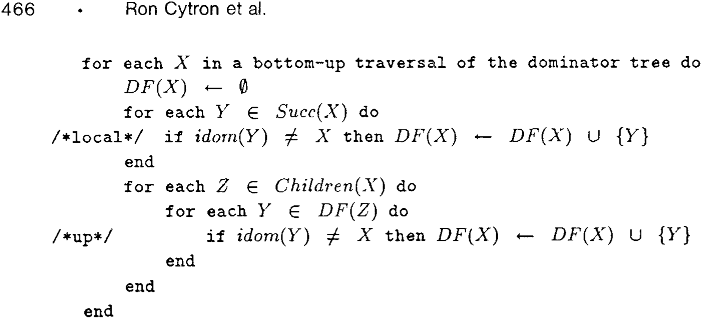
These results imply the correctness of the algorithm for computing the dominance frontiers given in Figure 10. The /local/ line effectively computes on the fly and uses it in (4) without needing to devote storage to it. The /up/ line is similar for . We traverse the dominator tree bottom-up, visiting each node only after visiting each of its children. To illustrate the working of this algorithm, we have annotated the dominator tree in Figure 9 with the information [ ] and () brackets.
Theorem 1. The algorithm in Figure 10 is correct.
Proof. Direct from the preceding lemmas.
Let have nodes and edges. The loop over in Figure 10 examines each edge just once, so all executions of the /local/ line are complete in time . Similarly, all executions of the /up/ line are complete in time . The overall time is thus , which amounts to a worst-case complexity of . However, Section 8 shows that, in practice, the size of the mapping is usually linear. We have implemented this algorithm and have observed that it is faster than the standard data-flow computations in the PTRAN compiler [2].
4.3 Relating Dominance Frontiers to Joins
We start by stating more formally the nonrecursive characterization of where the -functions should be located. Given a set of nodes, the set of join nodes is defined to be the set of all nodes such that there are two nonnull paths that start at two distinct nodes in and converge at . The iterated join is the limit of the increasing sequence of sets of nodes
In particular, if happens to be the set of assignment nodes for a variable , then is the set of -function nodes for .
The join and iterated join operations map sets of nodes to sets of nodes. We extend the dominance frontier mapping from nodes to sets of nodes in the natural way:
As with join, the iterated dominance frontier is the limit of the increasing sequence of sets of nodes
The actual computation of is performed by the efficient worklist algorithm in Section 5.1; the formulation here is convenient for relating iterated dominance frontiers to iterated joins. If the set is the set of assignment nodes for a variable , then we will show that
(this equation depends on the fact that Entry is in ) and, hence, that the location of the -functions for can be computed by the worklist algorithm for computing that is given in Section 5.1.
The following lemmas do most of the work by relating dominance frontiers to joins:
Lemma 4. For any nonnull path p: in , there is a node on p that dominates . Moreover, unless dominates every node on p, the node can be chosen in .
Proof. If dominates every node on , then we just choose to get all the claimed properties of . We may assume that some of the nodes on are not dominated by . Let the sequence of nodes on be . For the smallest such that does not dominate , the predecessor is dominated by and so puts into . Thus, there are choices of with . Consider for the largest with . We will show that . Suppose not. Then , and there is a first with such that does not dominate . The predecessor is dominated by and so puts into . Thus, , contradicting the choice of .
Lemma 5. Let be two nodes in CFG, and suppose that nonnull paths and in CFG converge at . Then .
Proof. We consider three cases that are obviously exhaustive. In the first two cases, we prove that . Then we show that the first two cases are (unobviously) exhaustive because the third case leads to a contradiction. Let be from Lemma 4 for the path , with the sequence of nodes . Let be from Lemma 4 for the path , with the sequence of nodes .
Case 1. We suppose that is on and show that . By the definition of convergence (specifically, (3) in Section 2), . We may now assume that and dominates every node on . (Otherwise, Lemma 4 already asserts .) Because dominates the predecessor of but does not strictly dominate , we have .
Case 2. We suppose that is on , and show that , reasoning just as in Case 1.
Case 3. We derive a contradiction from the suppositions that is not on and is not on . Because but is not on , and, therefore, dominates all predecessors of . In particular, . But , so , and we continue inductively to show that for all . In particular, . On the other hand, by similar reasoning from the supposition that but is not on , we can show that . Two nodes cannot strictly dominate each other, so Case 3 is impossible.
Lemma 6. For any set of CFG nodes, .
Proof. We apply Lemma 5.
Lemma 7. For any set of CFG nodes such that Entry , .
Proof. Consider any and any . There is a path from to where all nodes before are dominated by . There is also a path from Entry to where none of the nodes are dominated by . The paths therefore converge at .
Theorem 2. The set of nodes that need -functions for any variable V is the iterated dominance frontier , where is the set of nodes with assignments to V.
Proof. By Lemma 6 and induction on in the definition of , we can show that
The induction step is as follows:
The node Entry is in , so Lemma 7 and another induction yield
The induction step is as follows:
The set of nodes that need -functions for is precisely , so (5) and (6) prove the theorem. □
5 CONSTRUCTION OF MINIMAL SSA FORM
5.1 Using Dominance Frontiers to Find Where -Functions Are Needed
The algorithm in Figure 11 inserts trivial -functions. The outer loop of this algorithm is performed once for each variable in the program. Several data structures are used:
— is the worklist of nodes being processed. In each iteration of this algorithm, is initialized to the set of nodes that contain assignments to . Each node in the worklist ensures that each node in receives a -function. Each iteration terminates when the worklist becomes empty. — is an array of flags, one flag for each node, where indicates whether has ever been added to during the current iteration of the outer loop. — is an array of flags, one for each node, where indicates whether a -function for has already been inserted at .
The flags and are independent. We need two flags because the property of assigning to is independent of the property of needing a -function for . The flags could have been implemented with just the values true and false, but this would require additional record keeping to reset any true flags between iterations, without the expense of looping over all the nodes. It is simpler to devote an integer to each flag and to test flags by comparing them with the current iteration count.
Let each node have original assignments to variables, where each ordinary assignment statement contributes the length of the tuple to . Counting assignments to variables is one of
              IterCount ← 0
for each node X do
    HasAlready(X) ← 0
    Work(X) ← 0
end
W ← ∅
for each variable V do
    IterCount ← IterCount + 1
    for each X ∈ A(V) do
        Work(X) ← IterCount
        W ← W ∪ {X}
    end
while W ≠ ∅ do
    take X from W
    for each Y ∈ DF(X) do
        if HasAlready(Y) < IterCount
            then do
                place ⟨ V ← φ(V, ..., V) ⟩ at Y
                HasAlready(Y) ← IterCount
                if Work(Y) < IterCount
                    then do
                        Work(Y) ← IterCount
                        W ← W ∪ {Y}
                    end
                end
            end
        end
    end
end
Fig. 11. Placement of -functions.
several measures of program size. By this measure, the program expands from size to size , where each -function placed at contributes 1 to . There is a similar expansion in the number of mentions of variables, from to , where each -function placed at contributes 1 plus the indegree of to .
Placing a -function at in Figure 11 has cost linear in the indegree of , so there is an contribution to the running time from the work done when . Replacing mentions of variables will contribute at least to the running time of any SSA translation algorithm, so the cost of placement can be ignored in analyzing the contribution of Figure 11 to the bound for the whole process. The cost of
The various measures relevant here are reviewed when the whole SSA translation process is summarized in Section 9.1.
initialization can be similarly ignored because it is subsumed by the cost of the dominance frontier calculation. What cannot be ignored is the cost of managing the worklist W. The statement take X from W in Figure 11 is performed times, and each time incurs a cost linear in because all are polled. The contribution of Figure 11 to the running time of the whole process is therefore . Sizing the output in the natural way as , we can also describe the contribution as , where the weighted average
emphasizes the dominance frontiers of nodes with many assignments. As Section 8 shows, the dominance frontiers are small in practice, and Figure 11 is effectively . This, in turn, is effectively .
5.2 Renaming
The algorithm in Figure 12 renames all mentions of variables. New variables denoted , where is an integer, are generated for each variable . Figure 12 begins a top-down traversal of the dominator tree by calling SEARCH at the root node Entry. The visit to a node processes the statements associated with the node in sequential order, starting with any -functions that may have been inserted. The processing of a statement requires work for only those variables actually mentioned in the statement. In contrast with Figure 11, we need a loop over all variables only when we initialize two arrays among the following data structures:
— is an array of stacks, one stack for each variable . The stacks can hold integers. The integer at the top of is used to construct the variable that should replace a use of . — is an array of integers, one for each variable . The counter value tells how many assignments to have been processed. —WhichPred() is an integer telling which predecessor of in is . The th operand of a -function in corresponds to the th predecessor of from the listing of the inedges of . —Each assignment statement has the form
where the right-hand side is a tuple of expressions and the left-hand side is a tuple of distinct target variables. These tuples change as mentions of variables are renamed, but the original target tuple is still remembered as . To minimize notation, a conditional branch is treated as an ordinary assignment to a special variable whose value indicates which edge the branch should follow. A real implementation would recognize that a conditional branch involves a little less work than a genuine assignment: The part of the processing can be omitted.
              for each variable V do
    C(V) ← 0
    S(V) ← EmptyStack
end
call SEARCH(Entry)
SEARCH() : for each statement in do if is an ordinary assignment then for each variable used in do replace use of by use of , where end for each in do replace by new in push onto end end / of first loop / for each do for each -function in do replace the -th operand in by where end end for each do call SEARCH(Y) end end for each assignment in do for each in do pop end end end SEARCH
Fig. 12 Renaming mentions of variables. The list of uses of grows with each replacement of by in a
The processing of an assignment statement considers the mentions of variables in . The simplest case is that of a target variable in the tuple . We need a new variable . By keeping a count of the number of assignments to that have already been processed, we can find an appropriate new variable by using and then incrementing . To facilitate renaming uses of in the future, we also push (which identifies ) onto a stack of (integers that identify) new variables replacing .
A subtler computation is needed for the right-hand side . Consider any variable used in ; that is, appears in at least one of the expressions in the tuple. We want to replace by , where is the target of the assignment that produces the value for actually used in . There are two subcases because may be either an ordinary assignment or a -function. Both subcases get from the top of the stack , but they inspect at different times in Figure 12. Lemma 10, introduced later in this section, shows that is correctly chosen in both subcases.
The correctness proof for renaming depends on results from Section 4 and on three more lemmas. We start by showing that it makes sense to speak of "the" assignment to a variable in the transformed program.
Lemma 8. Each new variable in the transformed program is a target of exactly one assignment.
Proof. Because the counter is incremented after processing each assignment to , there can be at most one assignment to . To show that there is at least one assignment to , we consider the two ways can be mentioned. If is mentioned on the LHS on an assignment, then there is nothing more to show. If the value of is used, on the other hand, then was true at the time when the algorithm renamed the old use of to a use of . At the earlier time when was pushed onto , it was pushed because an assignment to had just been changed to an assignment to .
A node may contain assignments to the variable that appeared in the original program or were introduced to receive the value of a -function for . Let denote the new variable in effect for after all statements in node have been considered by the first loop in Figure 12. Specifically, we consider the top of each stack at the end of this loop and define
If there are no assignments to in , then the top-down traversal ensures that is inherited from the closest dominator of that assigns to .
Lemma 9. For any variable and any CFG edge such that does not have a -function for ,
Proof. We may assume that . Because does not have a -function for , if a node has , then does not assign to a new variable derived from . We use this fact twice below.
By Lemma 2, , and, thus, does not assign to a new variable derived from . Let be the first node in the sequence that assigns to such a variable. Then
Because assigns to a new variable derived from , it follows that . But dominates a predecessor of , so strictly dominates . For any with , we get because and there is an edge . By the choice of implies that does not assign to a new variable derived from . Therefore,
and (8) follows from (9).
The preceding lemma helps establish Condition (3) in the definition of SSA form, but first we must extend so as to specify which new variable corresponds to just before and just after each statement . There is one iteration of the first loop in Figure 12 for . We consider the top of each stack just before and just after this iteration to define
In particular, if happens to be the last statement in block , then . If, on the other hand, is followed by another statement , then .
Lemma 10. Consider any control flow path in the transformed program and the same path in the original program. Consider any variable and any occurrence of a statement along the path. If is from the original program, then the value of just before executing in the original program is the same as the value of just before executing in the transformed program.
Proof. We use induction along the path. We consider the th statement executed along the path and assume that, for all , the th statement is either not from the original program or has each variable agreeing with just before . We assume that the th statement is from the original program and show that agrees with just before .
Case 1. Suppose that is not the first original statement in its basic block . Let be the statement just before in . By the induction hypothesis and the semantics of assignment, agrees with just after . Thus, agrees with just before .
Case 2. Suppose that is the first original statement in its basic block . Let be the edge followed by the control path. We claim that agrees with when control flows along this edge.
If , then is and does hold the entry value of . If , let be the last statement in . By the induction hypothesis and the semantics of assignment, agrees with
It could be a nominal Entry assignment or a -function.
just after T and, hence, with TopAfter(V, X) when control flows along X → Y.
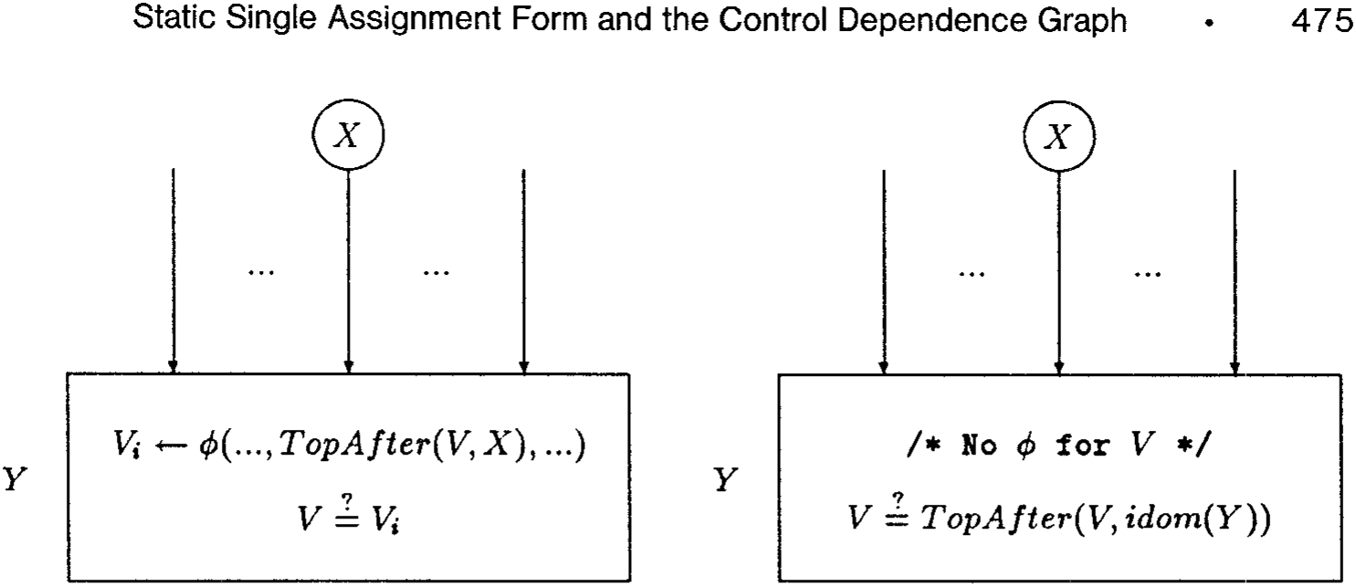
We must still bridge the gap between knowing that V agrees with TopAfter(V, X) along X → Y and knowing that V agrees with TopBefore(V, A) just before doing A in Y. As Figure 13 illustrates, there may or may not be a -function for V ahead of A in the transformed program.
Case 2.1. Suppose that V has a -function in Y. The operand corresponding to X → Y is TopAfter(V, X), thanks to the loop over successors of X in Figure 12. This is the operand whose value is assigned to , which is TopBefore(V, A). Thus, V agrees with TopBefore(V, A) just before doing A in Y.
Case 2.2. Suppose that V does not have a -function in Y. By Lemma 9, V agrees with TopAfter(V, X) = TopAfter(V, idom(Y)) = TopBefore(V, A) just before doing A in Y. □
Theorem 3. Any program can be put into minimal SSA form by computing the dominance frontiers and then applying the algorithms in Figure 11 and Figure 12. Let be the total number of assignments to variables in the resulting program.\footnote{Each ordinary assignment contributes the length of the tuple to , and each -function contributes 1 to .} Let be the total number of mentions of variables in the resulting program. Let E be the number of edges in CFG. Let avrgDF be the weighted average (7) of dominance frontier sizes. Then the running time of the whole process is
Proof. Figure 11 places the -functions for V at the nodes in the iterated dominance frontier , where is the set of assignments to V in the original program. By Theorem 2, is the set of nodes that need ϕ-functions for V, so we have obtained Condition (1) in the definition of translation to SSA form with the fewest possible ϕ-functions. We must still show that renaming is done correctly by Figure 12. Condition (2) in the definition follows from Lemma 8. Condition (3) follows from Lemma 10.
Let N be the number of nodes in CFG. The dominator tree has O(N) edges, and Figure 12 runs in time. The term is subsumed by the cost of computing the dominance frontiers, so Figure 12 contributes . As explained at the end of Section 5.1, Figure 11 contributes .
6 CONSTRUCTION OF CONTROL DEPENDENCIES
In this section we show that control dependences [24] are essentially the dominance frontiers in the reverse graph of the control flow graph. Let X and Y be nodes in CFG. If X appears on every path from Y to Exit, then X postdominates Y.8 Like the dominator relation, the postdominator relation is reflexive and transitive. If X postdominates Y but , then X strictly postdominates Y. The immediate postdominator of Y is the closest strict postdominator of Y on any path from Y to Exit. In a postdominator tree, the children of a node X are all immediately postdominated by X.
A CFG node Y is control dependent on a CFG node X if both of the following hold:
(1) There is a nonnull path such that Y postdominates every node after X on p. (2) The node Y does not strictly postdominate the node X.
In other words, there is some edge from X that definitely causes Y to execute, and there is also some path from X that avoids executing Y. We associate with this control dependence from X to Y the label on the control flow edge from X that causes Y to execute. Our definition of control dependence here can easily be shown to be equivalent to the original definition [24].
Lemma 11. Let X and Y be CFG nodes. Then Y postdominates a successor of X if and only if (iff) there is a nonnull path such that Y postdominates every node after X on p.
Proof. Suppose that Y postdominates a successor U of X. Choose any path q from U to Exit. Then Y appears on q. Let r be the initial segment of q that reaches the first appearance of Y on q. For any node V on r, we can get from U to Exit by following r to V and then by taking any path from V to Exit. Because Y postdominates U but does not appear before the end of r, Y must postdominate V as well. Let p be the path that starts with the edge and then proceeds along r. Then and Y postdominates every node after X on p.
8The postdominance relation in [24] is irreflexive, whereas the definition we use here is reflexive. The two relations are identical on pairs of distinct elements. We choose the reflexive definition here to make postdominance the dual of the dominance relation.
build build dominator tree for apply the algorithm in Figure 10 to find the dominance frontier mapping for
              for each node X do CD(X) ← ∅ end
for each node Y do
    for each X ∈ RDF(Y) do
        CD(X) ← CD(X) ∪ { Y }
    end
end
| Node | |
|---|---|
| Entry | 1,2,8,9,11,12 |
| 1 | |
| 2 | 3,6,7 |
| 3 | 4,5 |
| 4 | |
| 5 | |
| 6 | |
| 7 | |
| 8 | |
| 9 | 10 |
| 10 | |
| 11 | 9,11 |
| 12 | 2,8,9,11,12 |
Conversely, given a path with these properties, let be the first node after on . Then is a successor of and postdominates .
The reverse control flow graph has the same nodes as the control flow graph , but has an edge for each edge in . The roles of Entry and Exit are also reversed. The postdominator relation on is the dominator relation on .
Corollary 1. Let and be nodes in . Then is control dependent on in iff in .
Proof. Using Lemma 11 to simplify the first condition in the definition of control dependence, we find that is control dependent on iff postdominates a successor of but does not strictly postdominate . In this means that dominates a predecessor of but does not strictly dominate ; that is, .
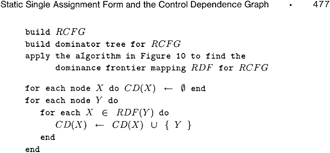
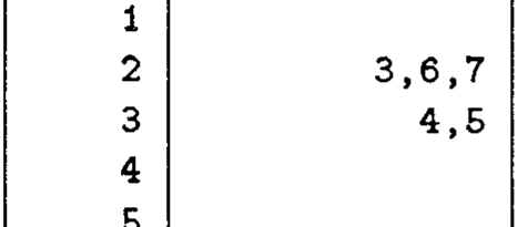
Figure 14 applies this result to the computation of control dependences. After building the dominator tree for by the standard method [35] in time , we spend finding dominance frontiers and then inverting them. The total time is thus for all practical purposes. By applying the algorithm in Figure 14 to the control flow graph in Figure 5, we obtain the control dependences in Figure 15. Note that the edge from Entry to Exit was added to so that the control dependence relation, viewed as a graph, would be rooted at Entry.
7 TRANSLATING FROM SSA FORM
Many powerful analysis and transformation techniques can be applied to programs in SSA form. Eventually, however, a program must be executed. The -functions have precise semantics, but they are generally not represented in existing target machines. This section describes how to translate out of SSA form by replacing each -function with some ordinary assignments. Naive translation could yield inefficient object code, but efficient code can be generated if two already useful optimizations are applied: dead code elimination and storage allocation by coloring.
Naively, a -input -function at entrance to a node can be replaced by ordinary assignments, one at the end of each control flow predecessor of . This is always correct, but these ordinary assignments sometimes perform a good deal of useless work. If the naive replacement is preceded by dead code elimination and then followed by coloring, however, the resulting code is efficient.
7.1 Dead Code Elimination
The original source program may have dead code (i.e., code that has no effect on any program output). Some of the intermediate steps in compilation (such as procedure integration) may also introduce dead code. Code that once was live may become dead in the course of optimization. With so many possible sources for dead code, it is natural to perform (or repeat) dead code elimination late in the optimization process, rather than burden many intermediate steps with concerns about dead code.
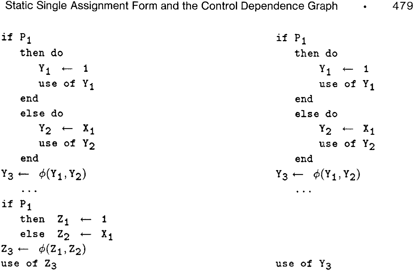
Translation to SSA form is one of the compilation steps that may introduce dead code. Suppose that is assigned and then used along each branch of an if...then...else..., but that is never used after the join point. The original assignments to are live, but the added assignment by the -function is dead. Often, such dead -functions are useful, as in the equivalencing and redundancy elimination algorithms that are based on SSA form [5, 43]. One such use is shown in Figure 16. Although others have avoided placement of dead -functions in translating to SSA form [16, 52], we prefer to include the dead -functions to increase optimization opportunities.
There are many different definitions of dead code in the literature. Dead code is sometimes defined to be unreachable code and sometimes defined (as it is here) to be ineffectual code. In both cases, it is desirable to use the broadest possible definition, subject to the correctness condition that "dead" code really can be safely removed.\footnote{The definition used here is broader than the usual one [1, p 595] and similar to that of "faint" variables [25, p. 489].} A procedural version of the definition is more intuitive than a recursive version, so we prefer the procedural style.
Initially, all statements are tentatively marked dead. Some statements, however, need to be marked live because of the conditions listed below. Marking these statements live may cause others to be marked live. When the natural worklist eventually empties, any statements that are still marked dead are truly dead and can be safely removed from the code.
              if P₁
then do
    Y₁ ← 1
    use of Y₁
end
else do
    Y₂ ← X₁
    use of Y₂
end
Y₃ ← φ(Y₁, Y₂)
...
if P₁
    then Z₁ ← 1
    else Z₂ ← X₁
Z₃ ← φ(Z₁, Z₂)
use of Z₃ if P₁
then do
    Y₁ ← 1
    use of Y₁
end
else do
    Y₂ ← X₁
    use of Y₂
end
Y₃ ← φ(Y₁, Y₂)
...
use of Y₃
A statement is marked live iff at least one of the following holds:
(1) The statement is one that should be assumed to affect program output, such as an I/O statement, an assignment to a reference parameter, or a call to a routine that may have side effects. (2) The statement is an assignment statement, and there are statements already marked live that use some of its outputs. (3) The statement is a conditional branch, and there are statements already marked live that are control dependent on this conditional branch.
Several published algorithms eliminate dead code in the narrower sense that requires every conditional branch to be marked live [30, 31, 38].¹⁰ Our algorithm, given in Figure 17, goes one step further in eliminating dead conditional branches. (An unpublished algorithm by R. Paige does this also.)
¹⁰ The more readily accessible [31] contains a typographical error; the earlier technical report [30] should be consulted for the correct version.
              for each statement S do
    if S ∈ PreLive
        then Live(S) ← true
        else Live(S) ← false
    end
WorkList ← PreLive
while () do take from WorkList
              for each D ∈ Definers(S) do
        if Live(D) = false
            then do
                Live(D) ← true
                WorkList ← WorkList ∪ { D }
            end
        end
    end

for each block B in CD⁻¹(Block(S)) do
        if Live(Last(B)) = false
            then do
                Live(Last(B)) ← true
                WorkList ← WorkList ∪ { Last(B) }
            end
        end
    end
end
for each statement do if false then delete from end
Fig. 17 Dead code elimination
The following data structures are used:
— indicates that statement is live. — is the set of statements whose execution is initially assumed to affect program output. Statements that result in I/O or side effects outside the current procedure scope are typically included. — is a list of statements whose liveness has been recently discovered. — is the set of statements that provide values used by statement . — is the statement that terminates basic block . — is the basic block containing statement . — is the basic block that immediately postdominates block .
— is the set of nodes that are control dependence predecessors of the node corresponding to block . This is the same as in Figure 14.
After the algorithm discovers the live statements, all those still not marked live are deleted. Other optimizations (such as code motion) may leave empty blocks, so there is already ample reason for a late optimization to remove them. The empty blocks left by dead code elimination can be removed along with any other empty blocks.
The fact that statements are considered dead until marked live is crucial for condition (2). Statements that depend (transitively) on themselves are never marked live unless required by some other live statement. Condition (3) is handled by the loop over . A basic block whose termination controls a block with live statements is itself live.
7.2 Allocation by Coloring
At first, it might seem possible simply to map all occurrences of back to and to delete all of the -functions. However, the new variables introduced by translation to SSA form cannot always be eliminated, because optimizations may have capitalized on the storage independence of the new variables. The useful persistence of the new variables introduced by translation to SSA form can be illustrated by the code motion example in Figure 18. The source code (Figure 18a) assigns to twice and uses it twice. The SSA form (Figure 18b) can be optimized by moving the invariant assignment out of the loop, yielding a program with separate variables for separate purposes (Figure 18c). The dead assignment to will be eliminated. These optimizations leave a region in the program where and are simultaneously live. Thus, both variables are required: The original variable cannot substitute for both renamed variables.
Any graph coloring algorithm [12, 13, 17, 18, 21] can be used to reduce the number of variables needed and thereby can remove most of the associated assignment statements. The choice of coloring technique should be guided by the eventual use of the output. If the goal is to produce readable source code, then it is desirable to consider each original variable separately, coloring just the SSA variables derived from . If the goal is machine code, then all of the SSA variables should be considered at once. In both cases, the process of coloring changes most of the assignments that were inserted to model the -functions into identity assignments, that is, assignments of the form . These identity assignments can all be deleted.
Storage savings are especially noticeable for arrays. If optimization does not perturb the order of the first two statements in Figure 7, then arrays and can be assigned the same color and, hence, can share the same storage. The array is then assigned an Update from an identically colored array. Such operations can be implemented inexpensively by assigning to just one component if the arrays share storage. In particular, the actual operation performed by HiddenUpdate is always of this form.
A conditional branch can be deleted by transforming it to an unconditional branch to any one of its prior targets.
              while (...) do    while (...) do    while (...) do
    W₃ ← φ(W₀, W₂)
    V₃ ← φ(V₀, V₂)
read V
read V_1
W \leftarrow V + W   W_1 \leftarrow V_1 + W_3
V \leftarrow 6      V_2 \leftarrow 6
W \leftarrow V + W   W_2 \leftarrow V_2 + W_1
end               end               end
(a)                (b)                (c)
Fig 18. Program that really uses two instances for a variable after code motion. (a) Source program; (b) unoptimized SSA form; (c) result of code motion.
8 ANALYSIS AND MEASUREMENTS
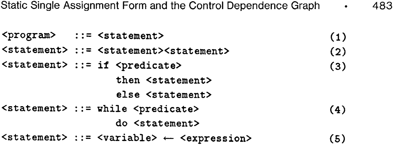
The number of nodes that contain -functions for a variable is a function of the program control flow structure and the assignments to . Program structure alone determines dominance frontiers and the number of control dependences. It is possible that dominance frontiers may be larger than necessary for computing -function locations for some programs, since the actual assignments are not taken into account. In this section we prove that the size of the dominance frontiers is linear in the size of the program when control flow branching is restricted to if-then-else constructs and while-do loops. (We assume that expressions and predicates perform no internal branching.) Such programs can be described by the grammar given in Figure 19. We also give experimental results that suggest that the behavior is linear for actual programs.
THEOREM 4. For programs comprised of straight-line code, if-then-else, and while-do constructs, the dominance frontier of any CFG node contains at most two nodes.
PROOF. Consider a top-down parse of a program using the grammar shown in Figure 19. Initially, we have a single node in the parse tree and a control flow graph with two nodes and one edge: Entry \rightarrow Exit. The initial dominance frontiers are . For each production, we consider the associated changes to and to the dominance frontiers of nodes. When a production expands a nonterminal parse tree node , a new subgraph is inserted into in place of . In this new subgraph, each node corresponds to a symbol on the right-hand side of the production.
We will show that applying any of the productions preserves the following invariants:
—Each node corresponding to an unexpanded symbol has at most one node in its dominance frontier.
              <program> ::= <statement>
<statement> ::= <statement><statement>
<statement> ::= if <predicate>
    then <statement>
    else <statement>
<statement> ::= while <predicate>
    do <statement>
<statement> ::= <variable> ← <expression>
—Each node corresponding to a terminal symbol has at most two nodes in its dominance frontier.
We consider the productions in turn.
(1) This production adds a node and edges Entry Exit, yielding .
(2) When this production is applied, a node is replaced by two nodes and . Edges previously entering and leaving now enter and leave . A single edge is inserted from to . Although the control flow graph has changed, consider how this production affects the dominator tree: Nodes and dominate all nodes that were dominated by ; additionally, dominates . Thus, we have .
(3) When this production is applied, a node is replaced by nodes , , , and . Edges previously entering and leaving now enter and leave . Edges are inserted from to both and ; edges are also inserted from and to . In the dominator tree, and both dominate all nodes that were dominated by . Additionally, dominates and . By the argument made for production (2), we have . Now consider nodes and . From the definition of a dominance frontier, we obtain .
(4) When this production is applied, a node is replaced by nodes and . All edges previously associated with node are now associated with node . Edges are inserted from to and from to . Node dominates all nodes that were dominated by node . Additionally, dominates . Thus, we have and .
(5) After application of this production, the new control flow graph is isomorphic to the old graph.
Corollary 2. For programs comprised of straight-line code, if-then-else, and while-do constructs, every node is control dependent on at most two nodes.
Proof. Consider a program composed of the allowed constructs and its associated control flow graph . The reverse control flow graph is
Table I. Summary Statistics of Our Experiment
              Package name  Statements in all procedures  Statements per procedure  Description
Min  Median  Max
EISPACK  7,034  22  89  327  Dense matrix eigenvectors and values
FLO52  2,054  9  54  351  Flow past an airfoil
SPICE  14,093  8  43  753  Circuit simulation
Totals  23,181  8  55  753  221 FORTRAN procedures
itself a structured control flow graph for some program . For all in contains at most two nodes by Theorem 4. By Corollary 1, is then control dependent on at most two nodes. □
Unfortunately, these linearity results do not hold for all program structures. In particular, consider the nest of repeat-until loops illustrated in Figure 5. For each loop, the dominance frontier of the entrance to that loop includes each of the entrances to surrounding loops. For nested loops, this leads to a dominance frontier mapping whose total size is , yet each variable needs at most -functions. Most of the dominance frontier mapping is not actually used in placing -functions, so it seems that the computation of dominance frontiers might take excessive time with respect to the resulting number of actual -functions. We therefore wish to measure the number of dominance frontier nodes as a function of program size over a diverse set of programs.
We implemented our algorithms for constructing dominance frontiers and placing -functions in the PTRAN system, which already offered the required local data flow and control flow analysis [2]. We ran these algorithms on 61 library procedures from EISPACK [46] and 160 procedures from two "Perfect" [39] benchmarks. Some summary statistics of these procedures are shown in Table I. These FORTRAN programs were chosen because they contain irreducible intervals and other unstructured constructs. As the plot in Figure 20 shows, the size of the dominance frontier mapping appears to vary linearly with program size. The ratio of these sizes ranged from 0.6 (the Entry node has an empty dominance frontier) to 2.1.
For the programs we tested, the plot in Figure 21 shows that the number of -functions is also linear in the size of the original program. The ratio of these sizes ranged from 0.5 to 5.2. The largest ratio occurred for a procedure of only 12 statements, and 95 percent of the procedures had a ratio under 2.3. All but one of the remaining procedures contained fewer than 60 statements. Finally, the plot in Figure 22 shows that the size of the control dependence graph is linear in the size of the original program. The ratio of these sizes ranged from 0.6 to 2.4, which is very close to the range of ratios for dominance frontiers.
The ratio (defined by (7) in Section 5.1) measures the cost of placing -functions relative to the number of assignments in the resulting
Fig. 20. Size of dominance frontier mapping versus number of program statements.
Fig. 21. Number of -functions versus number of program statements.
SSA form program. This ratio varied from 1 to 2, with median 1.3. There was no correlation with program size.
We also measured the expansion in the number of assignments when translating to SSA form. This ratio varied from 1.3 to 3.8. Finally, we measured the expansion in the number of mentions (assignments or uses) of variables when translating to SSA form. This ratio varied from 1.6 to 6.2. For both of these ratios, there was no correlation with program size.

9 DISCUSSION
9.1 Summary of Algorithms and Time Bounds
The conversion to SSA form is done in three steps:
(1) The dominance frontier mapping is constructed from the control flow graph (Section 4.2). Let have nodes and edges. Let be the mapping from nodes to their dominance frontiers. The time to compute the dominator tree and then the dominance frontiers in is .
(2) Using the dominance frontiers, the locations of the -functions for each variable in the original program are determined (Section 5.1). Let be the total number of assignments to variables in the resulting program, where each ordinary assignment statement contributes the length of the tuple to , and each -function contributes 1 to . Placing -functions contributes to the overall time, where is the weighted average (7) of the sizes .
(3) The variables are renamed (Section 5.2). Let be the total number of mentions of variables in the resulting program. Renaming contributes to the overall time.
To state the time bounds in terms of fewer parameters, let the overall size of the original program be the maximum of the relevant numbers: nodes, edges, original assignments to variables, and original mentions of variables. In the worst case, , and ordinary assignments can require insertions of -functions. Thus, at worst. In the worst case, a -function has operands. Thus, at worst. The one-parameter worst-case time bounds are thus for finding dominance frontiers and for translation to SSA form.
However, the data in Section 8 suggest that the entire translation to SSA form will be linear in practice. The dominance frontier of each node in is small, as is the number of -functions added for each variable. In effect, is constant, , and . The entire translation process is effectively .
Control dependences are read off from the dominance frontiers in the reverse graph (Section 6) in time . Since the size of is the size of the output of the control dependence calculation, this algorithm is linear in the size of the output. The only quadratic behavior is caused by the output being in the worst case. The data in Section 8 suggest that the control dependence calculation is effectively .
9.2 Related Work
Minimal SSA form is a refinement of Shapiro and Saint's [45] notion of a pseudoassignment. The pseudoassignment nodes for are exactly the nodes that need -functions for . A closer precursor [22] of SSA form associated new names for with pseudoassignment nodes and inserted assignments from one new name to another. Without explicit -functions, however, it was difficult to manage the new names or reason about the flow of values.
Suppose the control flow graph has nodes and edges for a program with variables. One algorithm [41] requires bit vector operations (where each vector is of length ) to find all of the pseudoassignments. A simpler algorithm [43] for reducible programs computes SSA form in time . With lengths of bit vectors taken into account, both of these algorithms are essentially on programs of size , and the simpler algorithm sometimes inserts extraneous -functions. The method presented here is at worst, but Section 8 gives evidence that it is in practice. The earlier algorithms have no provision for running faster in typical cases; they appear to be intrinsically quadratic.
For with nodes and edges, previous general control dependence algorithms [24] can take quadratic time in . This analysis is based on the worst-case depth of the (post)dominator tree [24, p. 326]. Section 6 shows that control dependences can be determined by computing dominance frontiers in the reverse graph . In general, our approach can also take quadratic time, but the only quadratic behavior is caused by the output being in the worst case. In particular, suppose a program is comprised only of straight-line code, if-then-else, and while-do constructs. By Corollary 2, our algorithm computes control dependences in linear time. We obtain a better time bound for such programs because our algorithm is based on dominance frontiers, whose sizes are not necessarily related to the depth of the dominator tree. For languages that offer only these constructs, control dependences can also be computed from the parse tree [28] in linear time, but our algorithm is more robust. It handles all cases in quadratic time and typical cases in linear time.
9.3 Conclusions
Previous work has shown that SSA form and control dependences can support powerful code optimization algorithms that are highly efficient in terms of time and space bounds based on the size of the program after translation to the forms. We have shown that this translation can be performed efficiently, that it leads to only a moderate increase in program size, and that applying the early steps in the SSA translation to the reverse graph is an efficient way to compute control dependences. This is strong evidence that SSA form and control dependences form a practical basis for optimization.
Acknowledgments
We would like to thank Fran Allen for early encouragement and Fran Allen, Trina Avery, Julian Padget, Bob Paige, Tom Reps, Randy Scarborough, and Jin-Fan Shaw for various helpful comments. We are especially grateful to the referees, whose thorough reports led to many improvements in this paper.