Gradient-based learning applied to document recognition Yann Lecun, Léon Bottou, Yoshua Bengio, Patrick Haffner
To cite this version: Yann Lecun, Léon Bottou, Yoshua Bengio, Patrick Haffner. Gradient-based learning applied to document recognition. Proceedings of the IEEE, 1998, 86 (11), pp.2278-2324. <10.1109/5.726791>. <hal-03926082>
HAL Id: hal-03926082 https://hal.science/hal-03926082v1 Submitted on 6 Jan 2023
HAL is a multi-disciplinary open access archive for the deposit and dissemination of scientific research documents, whether they are published or not. The documents may come from teaching and research institutions in France or abroad, or from public or private research centers.
L’archive ouverte pluridisciplinaire HAL, est destinée au dépôt et à la diffusion de documents scientifiques de niveau recherche, publiés ou non, émanant des établissements d’enseignement et de recherche français ou étrangers, des laboratoires publics ou privés.
HAL Authorization
Gradient-Based Learning Applied to Document Recognition
YANN LECUN, MEMBER, IEEE, LÉON BOTTOU, YOSHUA BENGIO, AND PATRICK HAFFNER
Multilayer neural networks trained with the back-propagation algorithm constitute the best example of a successful gradient-based learning technique. Given an appropriate network architecture, gradient-based learning algorithms can be used to synthesize a complex decision surface that can classify high-dimensional patterns, such as handwritten characters, with minimal preprocessing. This paper reviews various methods applied to handwritten character recognition and compares them on a standard handwritten digit recognition task. Convolutional neural networks, which are specifically designed to deal with the variability of two dimensional (2-D) shapes, are shown to outperform all other techniques.
Real-life document recognition systems are composed of multiple modules including field extraction, segmentation, recognition, and language modeling. A new learning paradigm, called graph transformer networks (GTN’s), allows such multimodule systems to be trained globally using gradient-based methods so as to minimize an overall performance measure.
Two systems for online handwriting recognition are described. Experiments demonstrate the advantage of global training, and the flexibility of graph transformer networks.
A graph transformer network for reading a bank check is also described. It uses convolutional neural network character recognizers combined with global training techniques to provide record accuracy on business and personal checks. It is deployed commercially and reads several million checks per day.
Keywords— Convolutional neural networks, document recognition, finite state transducers, gradient-based learning, graph transformer networks, machine learning, neural networks, optical character recognition (OCR).
Nomenclature
GT Graph transformer.
GTN Graph transformer network.
HMM Hidden Markov model.
HOS Heuristic oversegmentation.
K-NN K-nearest neighbor.
Y. LeCun, L. Bottou, and P. Haffner are with the Speech and Image Processing Services Research Laboratory, AT&T Labs-Research, Red Bank, NJ 07701 USA.
Y. Bengio is with the Département d’Informatique et de Recherche Opérationelle, Université de Montréal, Montréal, Québec H3C 3J7 Canada.
NN Neural network.
OCR Optical character recognition.
PCA Principal component analysis.
RBF Radial basis function.
RS-SVM Reduced-set support vector method.
SDNN Space displacement neural network.
SVM Support vector method.
TDNN Time delay neural network.
V-SVM Virtual support vector method.
I INTRODUCTION
Over the last several years, machine learning techniques, particularly when applied to NN’s, have played an increasingly important role in the design of pattern recognition systems. In fact, it could be argued that the availability of learning techniques has been a crucial factor in the recent success of pattern recognition applications such as continuous speech recognition and handwriting recognition.
The main message of this paper is that better pattern recognition systems can be built by relying more on automatic learning and less on hand-designed heuristics. This is made possible by recent progress in machine learning and computer technology. Using character recognition as a case study, we show that hand-crafted feature extraction can be advantageously replaced by carefully designed learning machines that operate directly on pixel images. Using document understanding as a case study, we show that the traditional way of building recognition systems by manually integrating individually designed modules can be replaced by a unified and well-principled design paradigm, called GTN’s, which allows training all the modules to optimize a global performance criterion.
Since the early days of pattern recognition it has been known that the variability and richness of natural data, be it speech, glyphs, or other types of patterns, make it almost impossible to build an accurate recognition system entirely by hand. Consequently, most pattern recognition systems are built using a combination of automatic learning techniques and hand-crafted algorithms. The usual method of recognizing individual patterns consists in dividing the system into two main modules shown in Fig. 1. The first module, called the feature extractor, transforms the input patterns so that they can be represented by low-dimensional vectors or short strings of symbols that: 1) can be easily matched or compared and 2) are relatively invariant with respect to transformations and distortions of the input patterns that do not change their nature. The feature extractor contains most of the prior knowledge and is rather specific to the task. It is also the focus of most of the design effort, because it is often entirely hand crafted. The classifier, on the other hand, is often general purpose and trainable. One of the main problems with this approach is that the recognition accuracy is largely determined by the ability of the designer to come up with an appropriate set of features. This turns out to be a daunting task which, unfortunately, must be redone for each new problem. A large amount of the pattern recognition literature is devoted to describing and comparing the relative merits of different feature sets for particular tasks.
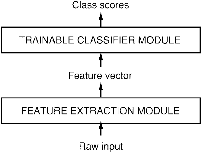
Historically, the need for appropriate feature extractors was due to the fact that the learning techniques used by the classifiers were limited to low-dimensional spaces with easily separable classes [1]. A combination of three factors has changed this vision over the last decade. First, the availability of low-cost machines with fast arithmetic units allows for reliance on more brute-force “numerical” methods than on algorithmic refinements. Second, the availability of large databases for problems with a large market and wide interest, such as handwriting recognition, has enabled designers to rely more on real data and less on hand-crafted feature extraction to build recognition systems. The third and very important factor is the availability of powerful machine learning techniques that can handle high-dimensional inputs and can generate intricate decision functions when fed with these large data sets. It can be argued that the recent progress in the accuracy of speech and handwriting recognition systems can be attributed in large part to an increased reliance on learning techniques and large training data sets. As evidence of this fact, a large proportion of modern commercial OCR systems use some form of multilayer NN trained with back propagation.
In this study, we consider the tasks of handwritten character recognition (Sections I and II) and compare the performance of several learning techniques on a benchmark data set for handwritten digit recognition (Section III). While more automatic learning is beneficial, no learning technique can succeed without a minimal amount of prior knowledge about the task. In the case of multilayer NN’s, a good way to incorporate knowledge is to tailor its architecture to the task. Convolutional NN’s [2], introduced in Section II, are an example of specialized NN architectures which incorporate knowledge about the invariances of two-dimensional (2-D) shapes by using local connection patterns and by imposing constraints on the weights. A comparison of several methods for isolated handwritten digit recognition is presented in Section III. To go from the recognition of individual characters to the recognition of words and sentences in documents, the idea of combining multiple modules trained to reduce the overall error is introduced in Section IV. Recognizing variable-length objects such as handwritten words using multinode systems is best done if the modules manipulate directed graphs. This leads to the concept of trainable GTN, also introduced in Section IV. Section V describes the now classical method of HOS for recognizing words or other character strings. Discriminative and nondiscriminative gradient-based techniques for training a recognizer at the word level without requiring manual segmentation and labeling are presented in Section VI. Section VII presents the promising space-displacement NN approach that eliminates the need for segmentation heuristics by scanning a recognizer at all possible locations on the input. In Section VIII, it is shown that trainable GTN’s can be formulated as multiple generalized transductions based on a general graph composition algorithm. The connections between GTN’s and HMM’s, commonly used in speech recognition, is also treated. Section IX describes a globally trained GTN system for recognizing handwriting entered in a pen computer. This problem is known as “online” handwriting recognition since the machine must produce immediate feedback as the user writes. The core of the system is a convolutional NN. The results clearly demonstrate the advantages of training a recognizer at the word level, rather than training it on presegmented, hand-labeled, isolated characters. Section X describes a complete GTN-based system for reading handwritten and machine-printed bank checks. The core of the system is the convolutional NN called LeNet-5, which is described in Section II. This system is in commercial use in the NCR Corporation line of check recognition systems for the banking industry. It is reading millions of checks per month in several banks across the United States.
A. Learning from Data
There are several approaches to automatic machine learning, but one of the most successful approaches, popularized in recent years by the NN community, can be called “numerical” or gradient-based learning. The learning machine computes a function where is the pth input pattern, and represents the collection of adjustable parameters in the system. In a pattern recognition setting, the output may be interpreted as the recognized class label of pattern , or as scores or probabilities associated with each class. A loss function measures the discrepancy between , the “correct” or desired output for pattern , and the output produced by the system. The average loss function is the average of the errors over a set of labeled examples called the training set . In the simplest setting, the learning problem consists in finding the value of that minimizes . In practice, the performance of the system on a training set is of little interest. The more relevant measure is the error rate of the system in the field, where it would be used in practice. This performance is estimated by measuring the accuracy on a set of samples disjoint from the training set, which is called the test set. Much theoretical and experimental work [3]–[5] has shown that the gap between the expected error rate on the test set and the error rate on the training set decreases with the number of training samples approximately as
where is the number of training samples, is a measure of “effective capacity” or complexity of the machine [6], [7], is a number between 0.5 and 1.0, and is a constant. This gap always decreases when the number of training samples increases. Furthermore, as the capacity increases, decreases. Therefore, when increasing the capacity , there is a tradeoff between the decrease of and the increase of the gap, with an optimal value of the capacity that achieves the lowest generalization error . Most learning algorithms attempt to minimize as well as some estimate of the gap. A formal version of this is called structural risk minimization [6], [7], and it is based on defining a sequence of learning machines of increasing capacity, corresponding to a sequence of subsets of the parameter space such that each subset is a superset of the previous subset. In practical terms, structural risk minimization is implemented by minimizing , where the function is called a regularization function and is a constant. is chosen such that it takes large values on parameters that belong to high-capacity subsets of the parameter space. Minimizing in effect limits the capacity of the accessible subset of the parameter space, thereby controlling the tradeoff between minimizing the training error and minimizing the expected gap between the training error and test error.
B. Gradient-Based Learning
The general problem of minimizing a function with respect to a set of parameters is at the root of many issues in computer science. Gradient-based learning draws on the fact that it is generally much easier to minimize a reasonably smooth, continuous function than a discrete (combinatorial) function. The loss function can be minimized by estimating the impact of small variations of the parameter values on the loss function. This is measured by the gradient of the loss function with respect to the parameters. Efficient learning algorithms can be devised when the gradient vector can be computed analytically (as opposed to numerically through perturbations). This is the basis of numerous gradient-based learning algorithms with continuous-valued parameters. In the procedures described in this article, the set of parameters is a real-valued vector, with respect to which is continuous, as well as differentiable almost everywhere. The simplest minimization procedure in such a setting is the gradient descent algorithm where is iteratively adjusted as follows:
In the simplest case, is a scalar constant. More sophisticated procedures use variable , or substitute it for a diagonal matrix, or substitute it for an estimate of the inverse Hessian matrix as in Newton or quasi-Newton methods. The conjugate gradient method [8] can also be used. However, Appendix B shows that despite many claims to the contrary in the literature, the usefulness of these second-order methods to large learning machines is very limited.
A popular minimization procedure is the stochastic gradient algorithm, also called the online update. It consists in updating the parameter vector using a noisy, or approximated, version of the average gradient. In the most common instance of it, is updated on the basis of a single sample
With this procedure the parameter vector fluctuates around an average trajectory, but usually it converges considerably faster than regular gradient descent and second-order methods on large training sets with redundant samples (such as those encountered in speech or character recognition). The reasons for this are explained in Appendix B. The properties of such algorithms applied to learning have been studied theoretically since the 1960’s [9]–[11], but practical successes for nontrivial tasks did not occur until the mid eighties.
C. Gradient Back Propagation
Gradient-based learning procedures have been used since the late 1950’s, but they were mostly limited to linear systems [1]. The surprising usefulness of such simple gradient descent techniques for complex machine learning tasks was not widely realized until the following three events occurred. The first event was the realization that, despite early warnings to the contrary [12], the presence of local minima in the loss function does not seem to be a major problem in practice. This became apparent when it was noticed that local minima did not seem to be a major impediment to the success of early nonlinear gradient-based learning techniques such as Boltzmann machines [13], [14]. The second event was the popularization by Rumelhart et al. [15] and others of a simple and efficient procedure to compute the gradient in a nonlinear system composed of several layers of processing, i.e., the back-propagation algorithm. The third event was the demonstration that the back-propagation procedure applied to multilayer NN’s with sigmoidal units can solve complicated learning tasks. The basic idea of back propagation is that gradients can be computed efficiently by propagation from the output to the input. This idea was described in the control theory literature of the early 1960’s [16], but its application to machine learning was not generally realized then. Interestingly, the early derivations of back propagation in the context of NN learning did not use gradients but “virtual targets” for units in intermediate layers [17], [18], or minimal disturbance arguments [19]. The Lagrange formalism used in the control theory literature provides perhaps the best rigorous method for deriving back propagation [20] and for deriving generalizations of back propagation to recurrent networks [21] and networks of heterogeneous modules [22]. A simple derivation for generic multilayer systems is given in Section I-E.
The fact that local minima do not seem to be a problem for multilayer NN’s is somewhat of a theoretical mystery. It is conjectured that if the network is oversized for the task (as is usually the case in practice), the presence of “extra dimensions” in parameter space reduces the risk of unattainable regions. Back propagation is by far the most widely used neural-network learning algorithm, and probably the most widely used learning algorithm of any form.
D. Learning in Real Handwriting Recognition Systems
Isolated handwritten character recognition has been extensively studied in the literature (see [23] and [24] for reviews), and it was one of the early successful applications of NN’s [25]. Comparative experiments on recognition of individual handwritten digits are reported in Section III. They show that NN’s trained with gradient-based learning perform better than all other methods tested here on the same data. The best NN’s, called convolutional networks, are designed to learn to extract relevant features directly from pixel images (see Section II).
One of the most difficult problems in handwriting recognition, however, is not only to recognize individual characters, but also to separate out characters from their neighbors within the word or sentence, a process known as segmentation. The technique for doing this that has become the “standard” is called HOS. It consists of generating a large number of potential cuts between characters using heuristic image processing techniques, and subsequently selecting the best combination of cuts based on scores given for each candidate character by the recognizer. In such a model, the accuracy of the system depends upon the quality of the cuts generated by the heuristics, and on the ability of the recognizer to distinguish correctly segmented characters from pieces of characters, multiple characters, or otherwise incorrectly segmented characters. Training a recognizer to perform this task poses a major challenge because of the difficulty in creating a labeled database of incorrectly segmented characters. The simplest solution consists of running the images of character strings through the segmenter and then manually labeling all the character hypotheses. Unfortunately, not only is this an extremely tedious and costly task, it is also difficult to do the labeling consistently. For example, should the right half of a cut-up four be labeled as a one or as a noncharacter? Should the right half of a cut-up eight be labeled as a three?
The first solution, described in Section V, consists of training the system at the level of whole strings of characters rather than at the character level. The notion of gradient-based learning can be used for this purpose. The system is trained to minimize an overall loss function which measures the probability of an erroneous answer. Section V explores various ways to ensure that the loss function is differentiable and therefore lends itself to the use of gradient-based learning methods. Section V introduces the use of directed acyclic graphs whose arcs carry numerical information as a way to represent the alternative hypotheses and introduces the idea of GTN.
The second solution, described in Section VII, is to eliminate segmentation altogether. The idea is to sweep the recognizer over every possible location on the input image, and to rely on the “character spotting” property of the recognizer, i.e., its ability to correctly recognize a well-centered character in its input field, even in the presence of other characters besides it, while rejecting images containing no centered characters [26], [27]. The sequence of recognizer outputs obtained by sweeping the recognizer over the input is then fed to a GTN that takes linguistic constraints into account and finally extracts the most likely interpretation. This GTN is somewhat similar to HMM’s, which makes the approach reminiscent of the classical speech recognition [28], [29]. While this technique would be quite expensive in the general case, the use of convolutional NN’s makes it particularly attractive because it allows significant savings in computational cost.
E. Globally Trainable Systems
As stated earlier, most practical pattern recognition systems are composed of multiple modules. For example, a document recognition system is composed of a field locator (which extracts regions of interest), a field segmenter (which cuts the input image into images of candidate characters), a recognizer (which classifies and scores each candidate character), and a contextual postprocessor, generally based on a stochastic grammar (which selects the best grammatically correct answer from the hypotheses generated by the recognizer). In most cases, the information carried from module to module is best represented as graphs with numerical information attached to the arcs. For example, the output of the recognizer module can be represented as an acyclic graph where each arc contains the label and the score of a candidate character, and where each path represents an alternative interpretation of the input string. Typically, each module is manually optimized, or sometimes trained, outside of its context. For example, the character recognizer would be trained on labeled images of presegmented characters. Then the complete system is assembled, and a subset of the parameters of the modules is manually adjusted to maximize the overall performance. This last step is extremely tedious, time consuming, and almost certainly suboptimal.
A better alternative would be to somehow train the entire system so as to minimize a global error measure such as the probability of character misclassifications at the document level. Ideally, we would want to find a good minimum of this global loss function with respect to all the parameters in the system. If the loss function measuring the performance can be made differentiable with respect to the system’s tunable parameters , we can find a local minimum of using gradient-based learning. However, at first glance, it appears that the sheer size and complexity of the system would make this intractable.
To ensure that the global loss function is differentiable, the overall system is built as a feedforward network of differentiable modules. The function implemented by each module must be continuous and differentiable almost everywhere with respect to the internal parameters of the module (e.g., the weights of an NN character recognizer in the case of a character recognition module), and with respect to the module’s inputs. If this is the case, a simple generalization of the well-known back-propagation procedure can be used to efficiently compute the gradients of the loss function with respect to all the parameters in the system [22]. For example, let us consider a system built as a cascade of modules, each of which implements a function , where is a vector representing the output of the module, is the vector of tunable parameters in the module (a subset of ), and is the module’s input vector (as well as the previous module’s output vector). The input to the first module is the input pattern . If the partial derivative of with respect to is known, then the partial derivatives of with respect to and can be computed using the backward recurrence
where is the Jacobian of with respect to evaluated at the point , and is the Jacobian of with respect to . The Jacobian of a vector function is a matrix containing the partial derivatives of all the outputs with respect to all the inputs. The first equation computes some terms of the gradient of , while the second equation generates a backward recurrence, as in the well-known back-propagation procedure for NN’s. We can average the gradients over the training patterns to obtain the full gradient. It is interesting to note that in many instances there is no need to explicitly compute the Jacobian matrix. The above formula uses the product of the Jacobian with a vector of partial derivatives, and it is often easier to compute this product directly without computing the Jacobian beforehand. In analogy with ordinary multilayer NN’s, all but the last module are called hidden layers because their outputs are not observable from the outside. In more complex situations than the simple cascade of modules described above, the partial derivative notation becomes somewhat ambiguous and awkward. A completely rigorous derivation in more general cases can be done using Lagrange functions [20]–[22].
Traditional multilayer NN’s are a special case of the above where the state information is represented with fixed-sized vectors, and where the modules are alternated layers of matrix multiplications (the weights) and component-wise sigmoid functions (the neurons). However, as stated earlier, the state information in complex recognition system is best represented by graphs with numerical information attached to the arcs. In this case, each module, called a GT, takes one or more graphs as input and produces a graph as output. Networks of such modules are called GTN’s. Sections IV, VI, and VIII develop the concept of GTN’s and show that gradient-based learning can be used to train all the parameters in all the modules so as to minimize a global loss function. It may seem paradoxical that gradients can be computed when the state information is represented by essentially discrete objects such as graphs, but that difficulty can be circumvented, as shown later.
II CONVOLUTIONAL NEURAL NETWORKS FOR ISOLATED CHARACTER RECOGNITION
The ability of multilayer networks trained with gradient descent to learn complex, high-dimensional, nonlinear mappings from large collections of examples makes them obvious candidates for image recognition tasks. In the traditional model of pattern recognition, a hand-designed feature extractor gathers relevant information from the input and eliminates irrelevant variabilities. A trainable classifier then categorizes the resulting feature vectors into classes. In this scheme, standard, fully connected multilayer networks can be used as classifiers. A potentially more interesting scheme is to rely as much as possible on learning in the feature extractor itself. In the case of character recognition, a network could be fed with almost raw inputs (e.g., size-normalized images). While this can be done with an ordinary fully connected feedforward network with some success for tasks such as character recognition, there are problems.
First, typical images are large, often with several hundred variables (pixels). A fully connected first layer with, e.g., one hundred hidden units in the first layer would already contain several tens of thousands of weights. Such a large number of parameters increases the capacity of the system and therefore requires a larger training set. In addition, the memory requirement to store so many weights may rule out certain hardware implementations. But the main deficiency of unstructured nets for image or speech applications is that they have no built-in invariance with respect to translations or local distortions of the inputs. Before being sent to the fixed-size input layer of an NN, character images, or other 2-D or one-dimensional (1-D) signals, must be approximately size normalized and centered in the input field. Unfortunately, no such preprocessing can be perfect: handwriting is often normalized at the word level, which can cause size, slant, and position variations for individual characters. This, combined with variability in writing style, will cause variations in the position of distinctive features in input objects. In principle, a fully connected network of sufficient size could learn to produce outputs that are invariant with respect to such variations. However, learning such a task would probably result in multiple units with similar weight patterns positioned at various locations in the input so as to detect distinctive features wherever they appear on the input. Learning these weight configurations requires a very large number of training instances to cover the space of possible variations. In convolutional networks, as described below, shift invariance is automatically obtained by forcing the replication of weight configurations across space.
Secondly, a deficiency of fully connected architectures is that the topology of the input is entirely ignored. The input variables can be presented in any (fixed) order without affecting the outcome of the training. On the contrary, images (or time-frequency representations of speech) have a strong 2-D local structure: variables (or pixels) that are spatially or temporally nearby are highly correlated. Local correlations are the reasons for the well-known advantages of extracting and combining local features before recognizing spatial or temporal objects, because configurations of neighboring variables can be classified into a small number of categories (e.g., edges, corners, etc.). Convolutional networks force the extraction of local features by restricting the receptive fields of hidden units to be local.
A. Convolutional Networks
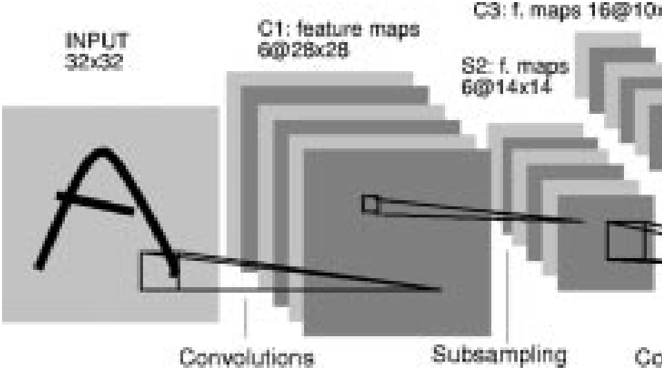
Convolutional networks combine three architectural ideas to ensure some degree of shift, scale, and distortion invariance: 1) local receptive fields; 2) shared weights (or weight replication); and 3) spatial or temporal subsampling. A typical convolutional network for recognizing characters, dubbed LeNet-5, is shown in Fig. 2. The input plane receives images of characters that are approximately size normalized and centered. Each unit in a layer receives inputs from a set of units located in a small neighborhood in the previous layer. The idea of connecting units to local receptive fields on the input goes back to the perceptron in the early 1960’s, and it was almost simultaneous with Hubel and Wiesel’s discovery of locally sensitive, orientation-selective neurons in the cat’s visual system [30]. Local connections have been used many times in neural models of visual learning [2], [18], [31]–[34]. With local receptive fields neurons can extract elementary visual features such as oriented edges, endpoints, corners (or similar features in other signals such as speech spectrograms). These features are then combined by the subsequent layers in order to detect higher order features. As stated earlier, distortions or shifts of the input can cause the position of salient features to vary. In addition, elementary feature detectors that are useful on one part of the image are likely to be useful across the entire image. This knowledge can be applied by forcing a set of units, whose receptive fields are located at different places on the image, to have identical weight vectors [15], [32], [34]. Units in a layer are organized in planes within which all the units share the same set of weights. The set of outputs of the units in such a plane is called a feature map. Units in a feature map are all constrained to perform the same operation on different parts of the image. A complete convolutional layer is composed of several feature maps (with different weight vectors), so that multiple features can be extracted at each location. A concrete example of this is the first layer of LeNet-5 shown in Fig. 2. Units in the first hidden layer of LeNet-5 are organized in six planes, each of which is a feature map. A unit in a feature map has 25 inputs connected to a area in the input, called the receptive field of the unit. Each unit has 25 inputs and therefore 25 trainable coefficients plus a trainable bias. The receptive fields of contiguous units in a feature map are centered on corresponding contiguous units in the previous layer. Therefore, receptive fields of neighboring units overlap. For example, in the first hidden layer of LeNet-5, the receptive fields of horizontally contiguous units overlap by four columns and five rows. As stated earlier, all the units in a feature map share the same set of 25 weights and the same bias, so they detect the same feature at all possible locations on the input. The other feature maps in the layer use different sets of weights and biases, thereby extracting different types of local features. In the case of LeNet-5, at each input location six different types of features are extracted by six units in identical locations in the six feature maps. A sequential implementation of a feature map would scan the input image with a single unit that has a local receptive field and store the states of this unit at corresponding locations in the feature map. This operation is equivalent to a convolution, followed by an additive bias and squashing function, hence the name convolutional network. The kernel of the convolution is the set of connection weights used by the units in the feature map. An interesting property of convolutional layers is that if the input image is shifted, the feature map output will be shifted by the same amount, but it will be left unchanged otherwise. This property is at the basis of the robustness of convolutional networks to shifts and distortions of the input.
Once a feature has been detected, its exact location becomes less important. Only its approximate position relative to other features is relevant. For example, once we know that the input image contains the endpoint of a roughly horizontal segment in the upper left area, a corner in the upper right area, and the endpoint of a roughly vertical segment in the lower portion of the image, we can tell the input image is a seven. Not only is the precise position of each of those features irrelevant for identifying the pattern, it is potentially harmful because the positions are likely to vary for different instances of the character. A simple way to reduce the precision with which the position of distinctive features are encoded in a feature map is to reduce the spatial resolution of the feature map. This can be achieved with a so-called subsampling layer, which performs a local averaging and a subsampling, thereby reducing the resolution of the feature map and reducing the sensitivity of the output to shifts and distortions. The second hidden layer of LeNet-5 is a subsampling layer. This layer comprises six feature maps, one for each feature map in the previous layer. The receptive field of each unit is a area in the previous layer’s corresponding feature map. Each unit computes the average of its four inputs, multiplies it by a trainable coefficient, adds a trainable bias, and passes the result through a sigmoid function. Contiguous units have nonoverlapping contiguous receptive fields. Consequently, a subsampling layer feature map has half the number of rows and columns as the feature maps in the previous layer. The trainable coefficient and bias control the effect of the sigmoid nonlinearity. If the coefficient is small, then the unit operates in a quasi-linear mode, and the subsampling layer merely blurs the input. If the coefficient is large, subsampling units can be seen as performing a “noisy OR” or a “noisy AND” function depending on the value of the bias. Successive layers of convolutions and subsampling are typically alternated resulting in a “bipyradid”: at each layer, the number of feature maps is increased as the spatial resolution is decreased. Each unit in the third hidden layer in Fig. 2 may have input connections from several feature maps in the previous layer. The convolution/subsampling combination, inspired by Hubel and Wiesel’s notions of “simple” and “complex” cells, was implemented in Fukushima’s Neocognitron [32], though no globally supervised learning procedure such as back propagation was available then. A large degree of invariance to geometric transformations of the input can be achieved with this progressive reduction of spatial resolution compensated by a progressive increase of the richness of the representation (the number of feature maps).
Since all the weights are learned with back propagation, convolutional networks can be seen as synthesizing their own feature extractor. The weight sharing technique has the interesting side effect of reducing the number of free parameters, thereby reducing the “capacity” of the machine and reducing the gap between test error and training error [34]. The network in Fig. 2 contains 345 308 connections, but only 60 000 trainable free parameters because of the weight sharing.
Fixed-size convolutional networks have been applied to many applications, among other handwriting recognition [35], [36], machine-printed character recognition [37], online handwriting recognition [38], and face recognition [39]. Fixed-size convolutional networks that share weights along a single temporal dimension are known as time-delay NN’s (TDNN’s). TDNN’s have been used in phoneme recognition (without subsampling) [40], [41], spoken word recognition (with subsampling) [42], [43], online recognition of isolated handwritten characters [44], and signature verification [45].
B. LeNet-5
This section describes in more detail the architecture of LeNet-5, the Convolutional NN used in the experiments. LeNet-5 comprises seven layers, not counting the input, all of which contain trainable parameters (weights). The input is a pixel image. This is significantly larger than the largest character in the database (at most pixels centered in a field). The reason is that it is desirable that potential distinctive features such as stroke endpoints or corner can appear in the center of the receptive field of the highest level feature detectors. In LeNet-5, the set of centers of the receptive fields of the last convolutional layer (C3, see below) form a area in the center of the input. The values of the input pixels are normalized so that the background level (white) corresponds to a value of and the foreground (black) corresponds to 1.175. This makes the mean input roughly zero and the variance roughly one, which accelerates learning [46].
In the following, convolutional layers are labeled Cx, subsampling layers are labeled Sx, and fully connected layers are labeled Fx, where x is the layer index.
Layer C1 is a convolutional layer with six feature maps. Each unit in each feature map is connected to a neighborhood in the input. The size of the feature maps is which prevents connection from the input from falling off the boundary. C1 contains 156 trainable parameters and 122 304 connections.
Layer S2 is a subsampling layer with six feature maps of size . Each unit in each feature map is connected to a neighborhood in the corresponding feature map in C1. The four inputs to a unit in S2 are added, then multiplied by
Table 1 Each Column Indicates Which Feature Map in S2 Are Combined by the Units in a Particular Feature Map of C3
| 0 | 1 | 2 | 3 | 4 | 5 | 6 | 7 | 8 | 9 | 10 | 11 | 12 | 13 | 14 | 15 | |
|---|---|---|---|---|---|---|---|---|---|---|---|---|---|---|---|---|
| 0 | X | X X X | X X X X | X X X X | X X | X X | X X | X X | X X | X X | X X | X X | X X | X X | X X | X X |
| 1 | X X | X X X | X X X X | X X X X | X X | X X | X X | X X | X X | X X | X X | X X | X X | X X | X X | X X |
| 2 | X X X | X X X | X X X X | X X X X | X X | X X | X X | X X | X X | X X | X X | X X | X X | X X | X X | X X |
| 3 | X X X | X X X X | X X X X | X X X X | X X | X X | X X | X X | X X | X X | X X | X X | X X | X X | X X | X X |
| 4 | X X X | X X X X | X X X X | X X X X | X X | X X | X X | X X | X X | X X | X X | X X | X X | X X | X X | X X |
| 5 | X X X | X X X X | X X X X | X X X X | X X | X X | X X | X X | X X | X X | X X | X X | X X | X X | X X | X X |
a trainable coefficient, and then added to a trainable bias. The result is passed through a sigmoidal function. The receptive fields are nonoverlapping, therefore feature maps in S2 have half the number of rows and column as feature maps in C1. Layer S2 has 12 trainable parameters and 5880 connections.
Layer C3 is a convolutional layer with 16 feature maps. Each unit in each feature map is connected to several neighborhoods at identical locations in a subset of S2’s feature maps. Table 1 shows the set of S2 feature maps combined by each C3 feature map. Why not connect every S2 feature map to every C3 feature map? The reason is twofold. First, a noncomplete connection scheme keeps the number of connections within reasonable bounds. More importantly, it forces a break of symmetry in the network. Different feature maps are forced to extract different (hopefully complementary) features because they get different sets of inputs. The rationale behind the connection scheme in Table 1 is the following. The first six C3 feature maps take inputs from every contiguous subsets of three feature maps in S2. The next six take input from every contiguous subset of four. The next three take input from some discontinuous subsets of four. Finally, the last one takes input from all S2 feature maps. Layer C3 has 1516 trainable parameters and 156 000 connections.
Layer S4 is a subsampling layer with 16 feature maps of size . Each unit in each feature map is connected to a neighborhood in the corresponding feature map in C3, in a similar way as C1 and S2. Layer S4 has 32 trainable parameters and 2000 connections.
Layer C5 is a convolutional layer with 120 feature maps. Each unit is connected to a neighborhood on all 16 of S4’s feature maps. Here, because the size of S4 is also , the size of C5’s feature maps is ; this amounts to a full connection between S4 and C5. C5 is labeled as a convolutional layer, instead of a fully connected layer, because if LeNet-5 input were made bigger with everything else kept constant, the feature map dimension would be larger than . This process of dynamically increasing the size of a convolutional network is described in Section VII. Layer C5 has 48 120 trainable connections.
Layer F6 contains 84 units (the reason for this number comes from the design of the output layer, explained below) and is fully connected to C5. It has 10 164 trainable parameters.
As in classical NN’s, units in layers up to F6 compute a dot product between their input vector and their weight vector, to which a bias is added. This weighted sum, denoted for unit , is then passed through a sigmoid squashing function to produce the state of unit , denoted by
The squashing function is a scaled hyperbolic tangent
where is the amplitude of the function and determines its slope at the origin. The function is odd, with horizontal asymptotes at and . The constant is chosen to be 1.7159. The rationale for this choice of a squashing function is given in Appendix A.
Finally, the output layer is composed of Euclidean RBF units, one for each class, with 84 inputs each. The outputs of each RBF unit is computed as follows:
In other words, each output RBF unit computes the Euclidean distance between its input vector and its parameter vector. The further away the input is from the parameter vector, the larger the RBF output. The output of a particular RBF can be interpreted as a penalty term measuring the fit between the input pattern and a model of the class associated with the RBF. In probabilistic terms, the RBF output can be interpreted as the unnormalized negative log-likelihood of a Gaussian distribution in the space of configurations of layer F6. Given an input pattern, the loss function should be designed so as to get the configuration of F6 as close as possible to the parameter vector of the RBF that corresponds to the pattern’s desired class. The parameter vectors of these units were chosen by hand and kept fixed (at least initially). The components of those parameters vectors were set to or . While they could have been chosen at random with equal probabilities for and , or even chosen to form an error correcting code as suggested by [47], they were instead designed to represent a stylized image of the corresponding character class drawn on a bitmap (hence the number 84). Such a representation is not particularly useful for recognizing isolated digits, but it is quite useful for recognizing strings of characters taken from the fully printable ASCII set. The rationale is that characters that are similar, and therefore confusable, such as uppercase “O,” lowercase “o,” and zero, lowercase “l” digit one, and square brackets and uppercase “I,” will have similar output codes. This is particularly useful if the system is combined with a linguistic post-processor that can correct such confusions. Because the codes for confusable classes are similar, the output of the corresponding RBF’s for an ambiguous character will be similar, and the postprocessor will be able to pick the appropriate interpretation. Fig. 3 gives the output codes for the full ASCII set.
Another reason for using such distributed codes, rather than the more common “1 of N” code (also called place code or grandmother cell code) for the outputs is that nondistributed codes tend to behave badly when the number of classes is larger than a few dozen. The reason is that output units in a nondistributed code must be off most of the time. This is quite difficult to achieve with sigmoid units. Yet another reason is that the classifiers are often used not only to recognize characters, but also to reject noncharacters. RBF’s with distributed codes are more appropriate for that purpose because unlike sigmoids, they are activated within a well-circumscribed region of their input space, outside of which nontypical patterns are more likely to fall.
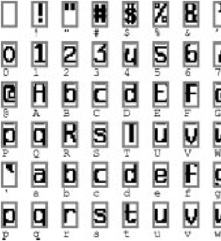
The parameter vectors of the RBF’s play the role of target vectors for layer F6. It is worth pointing out that the components of those vectors are +1 or −1, which is well within the range of the sigmoid of F6, and therefore prevents those sigmoids from getting saturated. In fact, +1 and −1 are the points of maximum curvature of the sigmoids. This forces the F6 units to operate in their maximally nonlinear range. Saturation of the sigmoids must be avoided because it is known to lead to slow convergence and ill-conditioning of the loss function.
C. Loss Function
The simplest output loss function that can be used with the above network is the maximum likelihood estimation criterion, which in our case is equivalent to the minimum mean squared error (MSE). The criterion for a set of training samples is simply
where is the output of the th RBF unit, i.e., the one that corresponds to the correct class of input pattern . While this cost function is appropriate for most cases, it lacks three important properties. First, if we allow the parameters of the RBF to adapt, has a trivial, but totally unacceptable, solution. In this solution, all the RBF parameter vectors are equal and the state of F6 is constant and equal to that parameter vector. In this case the network happily ignores the input, and all the RBF outputs are equal to zero. This collapsing phenomenon does not occur if the RBF weights are not allowed to adapt. The second problem is that there is no competition between the classes. Such a competition can be obtained by using a more discriminative training criterion, dubbed the maximum a posteriori (MAP) criterion, similar to maximum mutual information criterion sometimes used to train HMM’s [48]–[50]. It corresponds to maximizing the posterior probability of the correct class (or minimizing the logarithm of the probability of the correct class), given that the input image can come from one of the classes or from a background “rubbish” class label. In terms of penalties, it means that in addition to pushing down the penalty of the correct class like the MSE criterion, this criterion also pulls up the penalties of the incorrect classes
The negative of the second term plays a “competitive” role. It is necessarily smaller than (or equal to) the first term, therefore this loss function is positive. The constant is positive and prevents the penalties of classes that are already very large from being pushed further up. The posterior probability of this rubbish class label would be the ratio of and . This discriminative criterion prevents the previously mentioned “collapsing effect” when the RBF parameters are learned because it keeps the RBF centers apart from each other. In Section VI, we present a generalization of this criterion for systems that learn to classify multiple objects in the input (e.g., characters in words or in documents).
Computing the gradient of the loss function with respect to all the weights in all the layers of the convolutional network is done with back propagation. The standard algorithm must be slightly modified to take account of the weight sharing. An easy way to implement it is to first compute the partial derivatives of the loss function with respect to each connection, as if the network were a conventional multilayer network without weight sharing. Then the partial derivatives of all the connections that share a same parameter are added to form the derivative with respect to that parameter.
Such a large architecture can be trained very efficiently, but doing so requires the use of a few techniques that are described in the appendixes. Appendix A describes details such as the particular sigmoid used and the weight initialization. Appendixes B and C describe the minimization procedure used, which is a stochastic version of a diagonal approximation to the Levenberg–Marquardt procedure.
III RESULTS AND COMPARISON WITH OTHER METHODS
While recognizing individual digits is only one of many problems involved in designing a practical recognition system, it is an excellent benchmark for comparing shape recognition methods. Though many existing methods combine a hand-crafted feature extractor and a trainable classifier, this study concentrates on adaptive methods that operate directly on size-normalized images.
A. Database: The Modified NIST Set
The database used to train and test the systems described in this paper was constructed from the NIST’s Special Database 3 and Special Database 1 containing binary images of handwritten digits. NIST originally designated SD-3 as their training set and SD-1 as their test set. However, SD-3 is much cleaner and easier to recognize than SD-1. The reason for this can be found on the fact that SD-3 was collected among Census Bureau employees, while SD-1 was collected among high-school students. Drawing sensible conclusions from learning experiments requires that the result be independent of the choice of training set and test among the complete set of samples. Therefore it was necessary to build a new database by mixing NIST’s datasets.
SD-1 contains 58 527 digit images written by 500 different writers. In contrast to SD-3, where blocks of data from each writer appeared in sequence, the data in SD-1 is scrambled. Writer identities for SD-1 are available and we used this information to unscramble the writers. We then split SD-1 in two: characters written by the first 250 writers went into our new training set. The remaining 250 writers were placed in our test set. Thus we had two sets with nearly 30 000 examples each. The new training set was completed with enough examples from SD-3, starting at pattern #0, to make a full set of 60 000 training patterns. Similarly, the new test set was completed with SD-3 examples starting at pattern #35 000 to make a full set with 60 000 test patterns. In the experiments described here, we only used a subset of 10 000 test images (5,000 from SD-1 and 5,000 from SD-3), but we used the full 60 000 training samples. The resulting database was called the modified NIST, or MNIST, dataset.
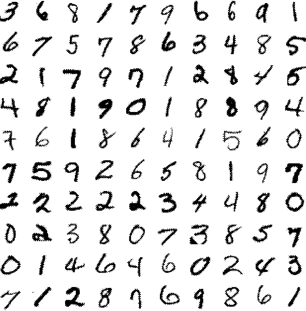
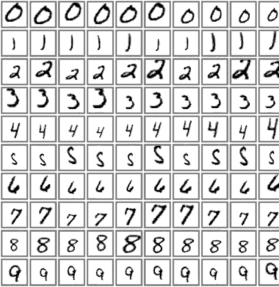
The original black and white (bilevel) images were size normalized to fit in a 20×20 pixel box while preserving their aspect ratio. The resulting images contain grey levels as result of the antialiasing (image interpolation) technique used by the normalization algorithm. Three versions of the database were used. In the first version, the images were centered in a 28×28 image by computing the center of mass of the pixels and translating the image so as to position this point at the center of the 28×28 field. In some instances, this 28×28 field was extended to 32×32 with background pixels. This version of the database will be referred to as the regular database. In the second version of the database, the character images were deslanted and cropped down to 20×20 pixels images. The deslanting computes the second moments of inertia of the pixels (counting a foreground pixel as one and a background pixel as zero) and shears the image by horizontally shifting the lines so that the principal axis is vertical. This version of the database will be referred to as the deslanted database. In the third version of the database, used in some early experiments, the images were reduced to 16×16 pixels.1 Fig. 4 shows examples randomly picked from the test set.
B. Results
Several versions of LeNet-5 were trained on the regular MNIST database. Twenty iterations through the entire training data were performed for each session. The values of the global learning rate [see (21) in Appendix C for a definition] was decreased using the following schedule: 0.0005 for the first two passes; 0.0002 for the next three; 0.0001 for the next three; 0.00005 for the next 4; and 0.00001 thereafter. Before each iteration, the diagonal
1 The regular database (60 000 training examples, 10 000 test examples size-normalized to 20×20 and centered by center of mass in 28×28 fields) is available WWW: http://www.research.att.com/˜yann/ocr/mnist.
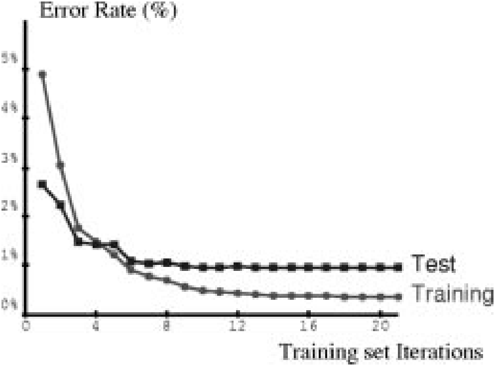
Hessian approximation was reevaluated on 500 samples, as described in Appendix C, and was kept fixed during the entire iteration. The parameter was set to 0.02. The resulting effective learning rates during the first pass varied between approximately and 0.016 over the set of parameters. The test error rate stabilizes after around ten passes through the training set at 0.95%. The error rate on the training set reaches 0.35% after 19 passes. Many authors have reported observing the common phenomenon of overtraining when training NN’s or other adaptive algorithms on various tasks. When overtraining occurs, the training error keeps decreasing over time but the test error goes through a minimum and starts increasing after a certain number of iterations. While this phenomenon is very common, it was not observed in our case as the learning curves in Fig. 5 show. A possible reason is that the learning rate was kept relatively large. The effect of this is that the weights never settle down in the local minimum but keep oscillating randomly. Because of those fluctuations, the average cost will be lower in a broader minimum. Therefore, stochastic gradient will have a similar effect as a regularization term that favors broader minima. Broader minima correspond to solutions with large entropy of the parameter distribution, which is beneficial to the generalization error.
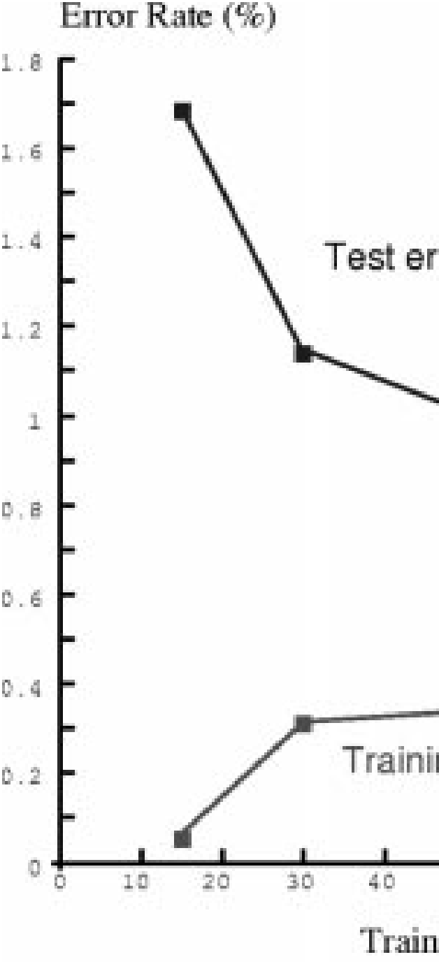
The influence of the training set size was measured by training the network with 15 000, 30 000, and 60 000 examples. The resulting training error and test error are shown in Fig. 6. It is clear that, even with specialized architectures such as LeNet-5, more training data would improve the accuracy.
To verify this hypothesis, we artificially generated more training examples by randomly distorting the original training images. The increased training set was composed of the 60 000 original patterns plus 540 000 instances of distorted patterns with randomly picked distortion parameters.
The distortions were combinations of the following planar affine transformations: horizontal and vertical translations; scaling; squeezing (simultaneous horizontal compression and vertical elongation, or the reverse); and horizontal shearing. Fig. 7 shows examples of distorted patterns used for training. When distorted data were used for training, the test error rate dropped to 0.8% (from 0.95% without deformation). The same training parameters were used as without deformations. The total length of the training session was left unchanged (20 passes of 60 000 patterns each). It is interesting to note that the network effectively sees each individual sample only twice over the course of these 20 passes.
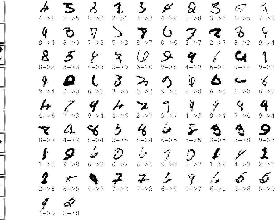
Fig. 8 shows all 82 misclassified test examples. some of those examples are genuinely ambiguous, but several are perfectly identifiable by humans, although they are written in an under-represented style. This shows that further improvements are to be expected with more training data.
C. Comparison with Other Classifiers
For the sake of comparison, a variety of other trainable classifiers was trained and tested on the same database. An early subset of these results was presented in [51]. The error rates on the test set for the various methods are shown in Fig. 9.
- Linear Classifier and Pairwise Linear Classifier: Possibly the simplest classifier that one might consider is a linear classifier. Each input pixel value contributes to a weighted sum for each output unit. The output unit with the highest sum (including the contribution of a bias constant) indicates the class of the input character. On the regular data, the error rate is 12%. The network has 7850 free parameters. On the deslanted images, the test error rate is 8.4%. The network has 4010 free parameters. The deficiencies of the linear classifier are well documented [1], and it is included here simply to form a basis of comparison for more sophisticated classifiers. Various combinations of sigmoid units, linear units, gradient descent learning, and learning by directly solving linear systems gave similar results.
A simple improvement of the basic linear classifier was tested [52]. The idea is to train each unit of a single-layer network to separate each class from each other class. In our case this layer comprises 45 units labeled 0/1, 0/2, ..., 0/9, 1/2, ..., 8/9. Unit i/j is trained to produce +1 on patterns of class i, -1 on patterns of class j,, and it is not trained on other patterns. The final score for class i is the sum of the outputs all the units labeled i/x minus the sum of the output of all the units labeled y/i, for all x and y. The error rate on the regular test set was 7.6%.
- Baseline Nearest Neighbor Classifier: Another simple classifier is a K-NN classifier with a Euclidean distance measure between input images. This classifier has the advantage that no training time, and no thought on the part of the designer, are required. However the memory requirement and recognition time are large: the complete 60 000 20 × 20 pixel training images (about 24 megabytes at one byte per pixel) must be available at run time. Much
more compact representations could be devised with modest increase in error rate. On the regular test set the error rate was 5.0%. On the deslanted data, the error rate was 2.4%, with . Naturally, a realistic Euclidean distance nearest-neighbor system would operate on feature vectors rather than directly on the pixels, but since all of the other systems presented in this study operate directly on the pixels, this result is useful for a baseline comparison.
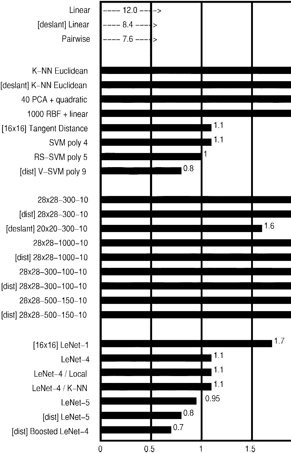
- PCA and Polynomial Classifier: Following [53] and [54], a preprocessing stage was constructed which computes the projection of the input pattern on the 40 principal components of the set of training vectors. To compute the principal components, the mean of each input component was first computed and subtracted from the training vectors. The covariance matrix of the resulting vectors was then computed and diagonalized using singular value decomposition. The 40-dimensional feature vector was used as the input of a second degree polynomial classifier. This classifier can be seen as a linear classifier with 821 inputs, preceded by a module that computes all products of pairs of input variables. The error on the regular test set was 3.3%.
- RBF Network: Following [55], an RBF network was constructed. The first layer was composed of 1000 Gaussian RBF units with 28×28 inputs, and the second layer was a simple 1000 inputs/ten outputs linear classifier. The RBF units were divided into ten groups of 100. Each group of units was trained on all the training examples of one of the ten classes using the adaptive K-means algorithm. The second-layer weights were computed using a regularized pseudoinverse method. The error rate on the regular test set was 3.6%.
- One-Hidden-Layer Fully Connected Multilayer NN: Another classifier that we tested was a fully connected multilayer NN with two layers of weights (one hidden layer) trained with the version of back-propagation described in Appendix C. Error on the regular test set was 4.7% for a network with 300 hidden units and 4.5% for a network with 1000 hidden units. Using artificial distortions to generate more training data brought only marginal improvement: 3.6% for 300 hidden units and 3.8% for 1000 hidden units. When deslanted images were used, the test error jumped down to 1.6% for a network with 300 hidden units.
It remains somewhat of a mystery that networks with such a large number of free parameters manage to achieve reasonably low testing errors. We conjecture that the dynamics of gradient descent learning in multilayer nets has a “self-regularization” effect. Because the origin of weight space is a saddle point that is attractive in almost every direction, the weights invariably shrink during the first few epochs (recent theoretical analysis seem to confirm this [56]). Small weights cause the sigmoids to operate in the quasi-linear region, making the network essentially equivalent to a low-capacity, single-layer network. As the learning proceeds the weights grow, which progressively increases the effective capacity of the network. This seems to be an almost perfect, if fortuitous, implementation of Vapnik’s “structural risk minimization” principle [6]. A better theoretical understanding of these phenomena, and more empirical evidence, are definitely needed.
- Two-Hidden-Layer Fully Connected Multilayer NN: To see the effect of the architecture, several two-hidden-layer multilayer NN’s were trained. Theoretical results have shown that any function can be approximated by a one-hidden-layer NN [57]. However, several authors have observed that two-hidden-layer architectures sometimes yield better performance in practical situations. This phenomenon was also observed here. The test error rate of a 28×28-300-100-10 network was 3.05%, a much better result than the one-hidden-layer network, obtained using marginally more weights and connections. Increasing the network size to 28×28-1000-150-10 yielded only marginally improved error rates: 2.95%. Training with distorted patterns improved the performance somewhat: 2.50% error for the 28×28-300-100-10 network, and 2.45% for the 28×28-1000-150-10 network.
- A Small Convolutional Network—LeNet-1: Convolutional networks are an attempt to solve the dilemma between small networks that cannot learn the training set and large networks that seem overparameterized. LeNet-1 was an early embodiment of the convolutional network architecture which is included here for comparison purposes. The images were down-sampled to 16×16 pixels and centered in the 28×28 input layer. Although about 100 000 multiply/add steps are required to evaluate LeNet-1, its convolutional nature keeps the number of free parameters to only about 2600. The LeNet-1 architecture was developed using our own version of the USPS (U.S. Postal Service zip codes) database and its size was tuned to match the available data [35]. LeNet-1 achieved 1.7% test error. The fact that a network with such a small number of parameters can attain such a good error rate is an indication that the architecture is appropriate for the task.
- LeNet-4: Experiments with LeNet-1 made it clear that a larger convolutional network was needed to make optimal use of the large size of the training set. LeNet-4 and later LeNet-5 were designed to address this problem. LeNet-4 is very similar to LeNet-5, except for the details of the architecture. It contains four first-level feature maps, followed by eight subsampling maps connected in pairs to each first-layer feature maps, then 16 feature maps, followed by 16 subsampling maps, followed by a fully connected layer with 120 units, followed by the output layer (ten units). LeNet-4 contains about 260 000 connections and has about 17 000 free parameters. Test error was 1.1%. In a series of experiments, we replaced the last layer of LeNet-4 with a Euclidean nearest-neighbor classifier, and with the “local learning” method of Bottou and Vapnik [58], in which a local linear classifier is retrained each time a new test pattern is shown. Neither of those methods improved the raw error rate, although they did improve the rejection performance.
- Boosted LeNet-4: Following theoretical work by Schapire [59], Drucker et al. [60] developed the “boosting” method for combining multiple classifiers. Three LeNet-4’s are combined: the first one is trained the usual way; the second one is trained on patterns that are filtered by the first net so that the second machine sees a mix of patterns, 50% of which the first net got right and 50% of which it got wrong; the third net is trained on new patterns on which the first and the second nets disagree. During testing, the outputs of the three nets are simply added. Because the error rate of LeNet-4 is very low, it was necessary to use the artificially distorted images (as with LeNet-5) in order to get enough samples to train the second and third nets. The test error rate was 0.7%, the best of any of our classifiers. At first glance, boosting appears to be three times more expensive as a single net. In fact, when the first net produces a high confidence answer, the other nets are not called. The average computational cost is about 1.75 times that of a single net.
- Tangent Distance Classifier: The tangent distance classifier is a nearest-neighbor method where the distance function is made insensitive to small distortions and translations of the input image [61]. If we consider an image as a point in a high-dimensional pixel space (where the dimensionality equals the number of pixels), then an evolving distortion of a character traces out a curve in pixel space. Taken together, all these distortions define a low-dimensional manifold in pixel space. For small distortions in the vicinity of the original image, this manifold can be approximated by a plane, known as the tangent plane. An excellent measure of “closeness” for character images is the distance between their tangent planes, where the set of distortions used to generate the planes includes translations, scaling, skewing, squeezing, rotation, and line thickness variations. A test error rate of 1.1% was achieved using 16×16 pixel images. Prefiltering techniques using simple Euclidean distance at multiple resolutions allowed to reduce the number of necessary tangent distance calculations.
- SVM: Polynomial classifiers are well studied methods for generating complex decision surfaces. Unfortunately, they are impractical for high-dimensional problems because the number of product terms is prohibitive. The support vector technique is an extremely economical way of representing complex surfaces in high-dimensional spaces, including polynomials and many other types of surfaces [6].
A particularly interesting subset of decision surfaces is the ones that correspond to hyperplanes that are at a maximum distance from the convex hulls of the two classes in the high-dimensional space of the product terms. Boser et al. [62] realized that any polynomial of degree k in this “maximum margin” set can be computed by first computing the dot product of the input image with a subset of the training samples (called the “support vectors”), elevating the result to the kth power, and linearly combining the numbers thereby obtained. Finding the support vectors and the coefficients amounts to solving a high-dimensional quadratic minimization problem with linear inequality constraints. For the sake of comparison, we include here the results
obtained by Burges and Schölkopf and reported in [63]. With a regular SVM, their error rate on the regular test set was 1.4%. Cortes and Vapnik had reported an error rate of 1.1% with SVM on the same data using a slightly different technique. The computational cost of this technique is very high: about 14 million multiply-adds per recognition. Using Schölkopf’s V-SVM technique, 1.0% error was attained. More recently, Schölkopf (personal communication) has reached 0.8% using a modified version of the V-SVM. Unfortunately, V-SVM is extremely expensive: about twice as much as regular SVM. To alleviate this problem, Burges has proposed the RS-SVM technique, which attained 1.1% on the regular test set [63], with a computational cost of only 650 000 multiply-adds per recognition, i.e., only about 60% more expensive than LeNet-5.
D. Discussion
A summary of the performance of the classifiers is shown in Figs. 9–12. Fig. 9 shows the raw error rate of the classifiers on the 10 000 example test set. Boosted LeNet-4 performed best, achieving a score of 0.7%, closely followed by LeNet-5 at 0.8%.
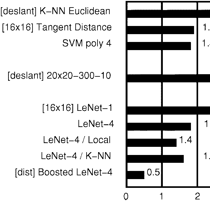
Fig. 10 shows the number of patterns in the test set that must be rejected to attain a 0.5% error for some of the methods. Patterns are rejected when the value of the corresponding output is smaller than a predefined threshold. In many applications, rejection performance is more significant than raw error rate. The score used to decide upon the rejection of a pattern was the difference between the scores of the top two classes. Again, Boosted LeNet-4 has the best performance. The enhanced versions of LeNet-4 did better than the original LeNet-4, even though the raw accuracies were identical.
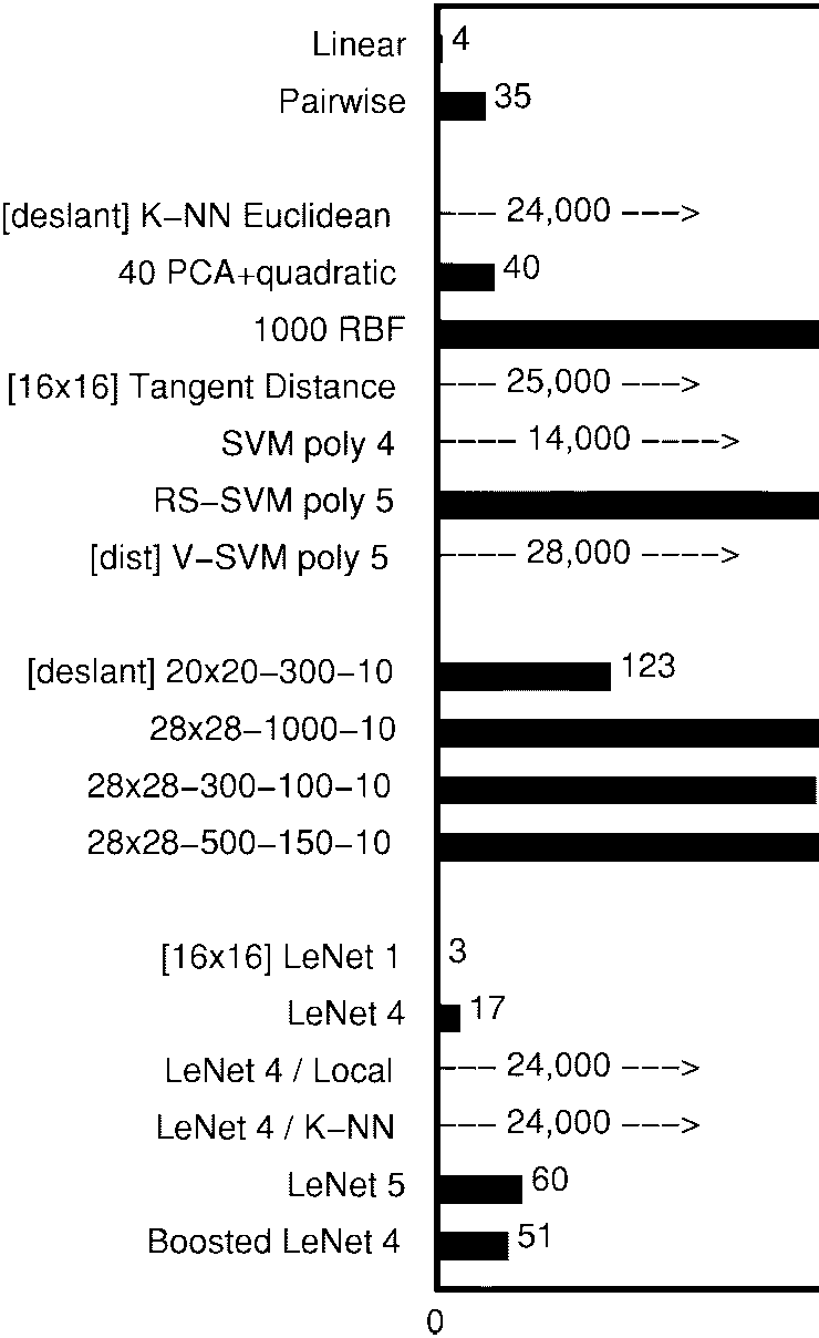
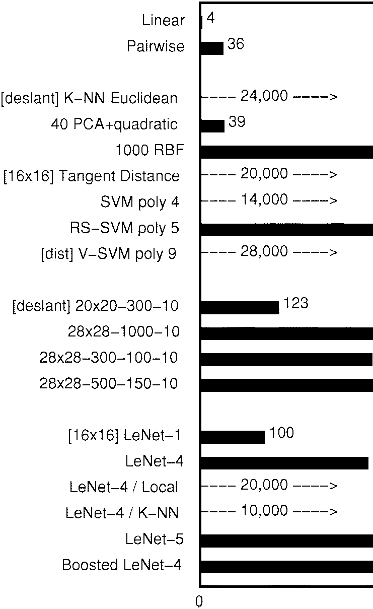
Fig. 11 shows the number of multiply–accumulate operations necessary for the recognition of a single size-normalized image for each method. Expectedly, NN’s are much less demanding than memory-based methods. Convolutional NN’s are particularly well suited to hardware implementations because of their regular structure and their low memory requirements for the weights. Single chip mixed analog–digital implementations of LeNet-5’s predecessors have been shown to operate at speeds in excess of 1000 characters per second [64]. However, the rapid progress of mainstream computer technology renders those exotic technologies quickly obsolete. Cost-effective implementations of memory-based techniques are more elusive due to their enormous memory requirements and computational requirements.
Training time was also measured. K-NN’s and tangent distance classifier have essentially zero training time. While the single-layer net, the pairwise net, and PCA+quadratic net could be trained in less than an hour, the multilayer net training times were expectedly much longer, but only required 10–20 passes through the training set. This amounts to two–three days of CPU to train LeNet-5 on a Silicon Graphics Origin 2000 server using a single 200 MHz R10000 processor. It is important to note that while the training time is somewhat relevant to the designer, it is of little interest to the final user of the system. Given the choice between an existing technique and a new technique that brings marginal accuracy improvements at the price of considerable training time, any final user would choose the latter.
Fig. 12 shows the memory requirements, and therefore the number of free parameters, of the various classifiers measured in terms of the number of variables that need to be stored. Most methods require only about 1 byte per variable for adequate performance. However, nearest-neighbor methods may get by with 4 bits per pixel for storing the template images. Not surprisingly, NN’s require much less memory than memory-based methods.
The overall performance depends on many factors including accuracy, running time, and memory requirements. As computer technology improves, larger capacity recognizers become feasible. Larger recognizers in turn require larger training sets. LeNet-1 was appropriate to the available technology in 1989, just as LeNet-5 is appropriate now. In 1989 a recognizer as complex as LeNet-5 would have required several weeks’ training and more data than were available and was therefore not even considered. For quite a long time, LeNet-1 was considered the state of the art. The local learning classifier, the optimal margin classifier, and the tangent distance classifier were developed to improve upon LeNet-1—and they succeeded at that. However, they in turn motivated a search for improved NN architectures. This search was guided in part by estimates of the capacity of various learning machines, derived from measurements of the training and test error as a function of the number of training examples. We discovered that more capacity was needed. Through a series of experiments in architecture, combined with an analysis of the characteristics of recognition errors, LeNet-4 and LeNet-5 were crafted.
We find that boosting gives a substantial improvement in accuracy, with a relatively modest penalty in memory and computing expense. Also, distortion models can be used to increase the effective size of a data set without actually requiring to collect more data.
The SVM has excellent accuracy, which is most remarkable because, unlike the other high performance classifiers, it does not include a priori knowledge about the problem. In fact, this classifier would do just as well if the image pixels were permuted with a fixed mapping and lost their pictorial structure. However, reaching levels of performance comparable to the convolutional NN’s can only be done at considerable expense in memory and computational requirements. The RS-SVM requirements are within a factor of two of the convolutional networks, and the error rate is very close. Improvements of those results are expected as the technique is relatively new.
When plenty of data are available, many methods can attain respectable accuracy. The neural-net methods run much faster and require much less space than memory-based techniques. The NN’s advantage will become more striking as training databases continue to increase in size.
E. Invariance and Noise Resistance
Convolutional networks are particularly well suited for recognizing or rejecting shapes with widely varying size, position, and orientation, such as the ones typically produced by heuristic segmenters in real-world string recognition systems.
In an experiment like the one described above, the importance of noise resistance and distortion invariance is not obvious. The situation in most real applications is quite different. Characters generally must be segmented out of their context prior to recognition. Segmentation algorithms are rarely perfect and often leave extraneous marks in character images (noise, underlines, neighboring characters), or sometimes cut characters too much and produce incomplete characters. Those images cannot be reliably size-normalized and centered. Normalizing incomplete characters can be very dangerous. For example, an enlarged stray mark can look like a genuine “1.” Therefore, many systems have resorted to normalizing the images at the level of fields or words. In our case, the upper and lower profiles of entire fields (i.e., amounts in a check) are detected and used to normalize the image to a fixed height. While this guarantees that stray marks will not be blown up into character-looking images, this also creates wide variations of the size and vertical position of characters after segmentation. Therefore it is preferable to use a recognizer that is robust to such variations. Fig. 13 shows several examples of distorted characters that are correctly recognized by LeNet-5. It is estimated that accurate recognition occurs for scale variations up to about a factor of two, vertical shift variations of plus or minus about half the height of the character, and rotations up to plus or minus 30 degrees. While fully invariant recognition of complex shapes is still an elusive goal, it seems that convolutional networks offer a partial answer to the problem of invariance or robustness with respect to geometrical distortions.
Fig. 13 includes examples of the robustness of LeNet-5 under extremely noisy conditions. Processing those images would pose insurmountable problems of segmentation and feature extraction to many methods, but LeNet-5 seems able to robustly extract salient features from these cluttered images. The training set used for the network shown here was the MNIST training set with salt and pepper noise added. Each pixel was randomly inverted with probability 0.1.\footnote{More examples of LeNet-5 in action are available WWW: http://www.research.att.com/˜yann/ocr
IV MULTIMODULE SYSTEMS AND GRAPH TRANSFORMER NETWORKS
The classical back-propagation algorithm, as described and used in the previous sections, is a simple form of gradient-based learning. However, it is clear that the gradient back-propagation algorithm given by (4) describes a more general situation than simple multilayer feedforward networks composed of alternated linear transformations and sigmoidal functions. In principle, derivatives can be back-propagated through any arrangement of functional modules, as long as we can compute the product of the Jacobians of those modules by any vector. Why would we want to train systems composed of multiple heterogeneous modules? The answer is that large and complex trainable systems need to be built out of simple, specialized modules. The simplest example is LeNet-5, which mixes convolutional layers, subsampling layers, fully connected layers, and RBF layers. Another less trivial example, described in Sections IV-A and IV-B, is a system for recognizing words, that can be trained to simultaneously segment and recognize words without ever being given the correct segmentation.
Fig. 14 shows an example of a trainable multimodular system. A multimodule system is defined by the function implemented by each of the modules and by the graph of interconnection of the modules to each other. The graph implicitly defines a partial order according to which the modules must be updated in the forward pass. For example in Fig. 14, module 0 is first updated, then modules 1 and 2 are updated (possibly in parallel), followed by module 3. Modules may or may not have trainable parameters. Loss functions, which measure the performance of the system, are implemented as module 4. In the simplest case, the loss function module receives an external input that carries the desired output. In this framework, there is no qualitative difference between trainable parameters (W1,
Fig. 13. Examples of unusual, distorted, and noisy characters correctly recognized by LeNet-5. {#lecun-1998-lenet-fig-13 .figure tag=08B2} The grey level of the output label represents the penalty (lighter for higher penalties).
Complex modules can be constructed from simpler modules by simply defining a new class whose slots will contain the member modules and the intermediate state variables between those modules. The fprop method for the class simply calls the fprop methods of the member modules, with the appropriate intermediate state variables or external input and outputs as arguments. Although the algorithms are easily generalizable to any network of such modules, including those whose influence graph has cycles, we will limit the discussion to the case of directed acyclic graphs (feed-forward networks). Computing derivatives in a multimodule system is just as simple. A “backward propagation” method, called bprop, for each module class can be defined for that purpose. The bprop method of a module takes the same arguments as the fprop method. All the derivatives in the system can be computed by calling the bprop method on all the modules in reverse order compared to the forward propagation phase. The state variables are assumed to contain slots for storing the gradients computed during the backward pass, in addition to storage for the states computed in the forward pass. The backward pass effectively computes the partial derivatives of the loss with respect to all the state variables and all the parameters in the system. There is an interesting duality property between the forward and backward functions of certain modules. For example, a sum of several variables in the forward direction is transformed into a simple fan-out (replication) in the backward w2 in the figure), external inputs and outputs (), and intermediate state variables ().
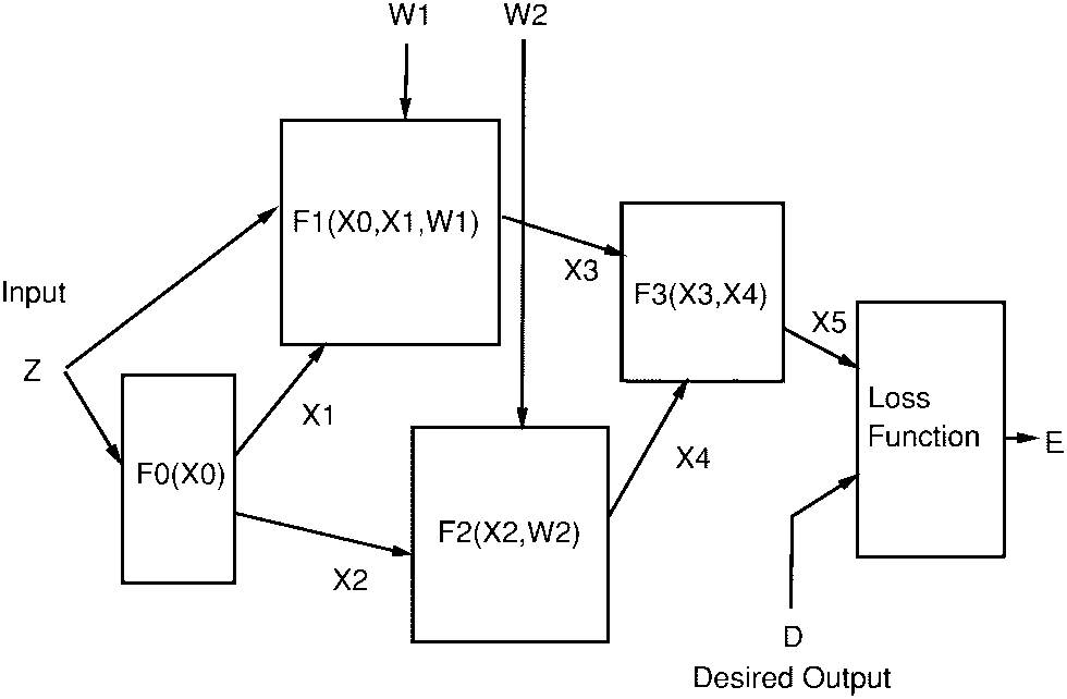
A. An Object-Oriented Approach
Object-oriented programming offers a particularly convenient way of implementing multimodule systems. Each module is an instance of a class. Module classes have a “forward propagation” method (or member function) called fprop whose arguments are the inputs and outputs of the module. For example, computing the output of module 3 in Fig. 14 can be done by calling the method fprop on module 3 with the arguments X3, X4, X5.
direction. Conversely, a fan-out in the forward direction is transformed into a sum in the backward direction. The software environment used to obtain the results described in this paper, called SN3.1, uses the above concepts. It is based on a home-grown object-oriented dialect of Lisp with a compiler to C.
The fact that derivatives can be computed by propagation in the reverse graph is easy to understand intuitively. The best way to justify it theoretically is through the use of Lagrange functions [21], [22]. The same formalism can be used to extend the procedures to networks with recurrent connections.
B. Special Modules
NN’s and many other standard pattern recognition techniques can be formulated in terms of multimodular systems trained with gradient-based learning. Commonly used modules include matrix multiplications and sigmoidal modules, the combination of which can be used to build conventional NN’s. Other modules include convolutional layers, subsampling layers, RBF layers, and “softmax” layers [65]. Loss functions are also represented as modules whose single output produces the value of the loss. Commonly used modules have simple bprop methods. In general, the bprop method of a function is a multiplication by the Jacobian of . Here are a few commonly used examples. The bprop method of a fanout (a “Y” connection) is a sum, and vice versa. The bprop method of a multiplication by a coefficient is a multiplication by the same coefficient. The bprop method of a multiplication by a matrix is a multiplication by the transpose of that matrix. The bprop method of an addition with a constant is the identity.
Interestingly, certain nondifferentiable modules can be inserted in a multinode system without adverse effect. An interesting example of that is the multiplexer module. It has two (or more) regular inputs, one switching input, and one output. The module selects one of its inputs, depending upon the (discrete) value of the switching input, and copies it on its output. While this module is not differentiable with respect to the switching input, it is differentiable with respect to the regular inputs. Therefore the overall function of a system that includes such modules will be differentiable with respect to its parameters as long as the switching input does not depend upon the parameters. For example, the switching input can be an external input.
Another interesting case is the min module. This module has two (or more) inputs and one output. The output of the module is the minimum of the inputs. The function of this module is differentiable everywhere, except on the switching surface which is a set of measure zero. Interestingly, this function is continuous and reasonably regular, and that is sufficient to ensure the convergence of a gradient-based learning algorithm.
The object-oriented implementation of the multinode idea can easily be extended to include a bbprop method that propagates Gauss–Newton approximations of the second derivatives. This leads to a direct generalization for modular systems of the second-derivative back propagation (22) given in Appendix C.
The multiplexer module is a special case of a much more general situation, described at length in Section IX, where the architecture of the system changes dynamically with the input data. Multiplexer modules can be used to dynamically rewire (or reconfigure) the architecture of the system for each new input pattern.
C. GTN’s
Multimodule systems are very flexible tools for building a large trainable system. However, the descriptions in the previous sections implicitly assumed that the set of parameters, and the state information communicated between the modules, are all fixed-size vectors. The limited flexibility of fixed-size vectors for data representation is a serious deficiency for many applications, notably for tasks that deal with variable length inputs (e.g., continuous speech recognition and handwritten word recognition) or for tasks that require encoding relationships between objects or features whose number and nature can vary (invariant perception, scene analysis, recognition of composite objects). An important special case is the recognition of strings of characters or words.
More generally, fixed-size vectors lack flexibility for tasks in which the state must encode probability distributions over sequences of vectors or symbols, as is the case in linguistic processing. Such distributions over sequences are best represented by stochastic grammars, or, in the more general case, directed graphs in which each arc contains a vector (stochastic grammars are special cases in which the vector contains probabilities and symbolic information). Each path in the graph represents a different sequence of vectors. Distributions over sequences can be represented by interpreting elements of the data associated with each arc as parameters of a probability distribution or simply as a penalty. Distributions over sequences are particularly handy for modeling linguistic knowledge in speech or handwriting recognition systems: each sequence, i.e., each path in the graph, represents an alternative interpretation of the input. Successive processing modules progressively refine the interpretation. For example, a speech recognition system might start with a single sequence of acoustic vectors, transform it into a lattice of phonemes (distribution over phoneme sequences), then into a lattice of words (distribution over word sequences), and then into a single sequence of words representing the best interpretation.
In our work on building large-scale handwriting recognition systems, we have found that these systems could be developed and designed much more easily and quickly by viewing the system as a networks of modules that take one or several graphs as input and produce graphs as output. Such modules are called GT’s, and the complete systems are called GTN’s. Modules in a GTN communicate their states and gradients in the form of directed graphs whose arcs carry numerical information (scalars or vectors) [66].
From the statistical point of view, the fixed-size state vectors of conventional networks can be seen as representing the means of distributions in state space. In variable-size networks such as the space-displacement NN’s described in Section VII, the states are variable-length sequences of fixed size vectors. They can be seen as representing the mean of a probability distribution over variable-length sequences of fixed-size vectors. In GTN’s the states are represented as graphs, which can be seen as representing mixtures of probability distributions over structured collections (possibly sequences) of vectors (Fig. 15).
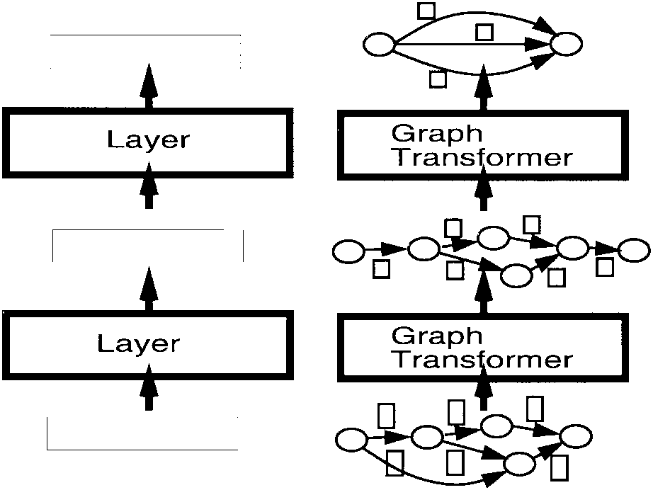
One of the main points of the next several sections is to show that gradient-based learning procedures are not limited to networks of simple modules that communicate through fixed-size vectors but can be generalized to GTN’s. Gradient back propagation through a GT takes gradients with respect to the numerical information in the output graph and computes gradients with respect to the numerical information attached to the input graphs, and with respect to the module’s internal parameters. Gradient-based learning can be applied as long as differentiable functions are used to produce the numerical data in the output graph from the numerical data in the input graph and the functions parameters.
The second point of the next several sections is to show that the functions implemented by many of the modules used in typical document processing systems (and other image recognition systems), though commonly thought to be combinatorial in nature, are indeed differentiable with respect to their internal parameters as well as with respect to their inputs, and are therefore usable as part of a globally trainable system.
In most of the following, we will purposely avoid making references to probability theory. All the quantities manipulated are viewed as penalties, or costs, which if necessary can be transformed into probabilities by taking exponentials and normalizing.
V MULTIPLE OBJECT RECOGNITION: HOS
One of the most difficult problems of handwriting recognition is to recognize not just isolated characters, but strings of characters such as zip codes, check amounts, or words. Since most recognizers can only deal with one character at a time, we must first segment the string into individual character images. However, it is almost impossible to devise image analysis techniques that will infallibly segment naturally written sequences of characters into well formed characters.
The recent history of automatic speech recognition [28], [67] is here to remind us that training a recognizer by optimizing a global criterion (at the word or sentence level) is much preferable to merely training it on hand-segmented phonemes or other units. Several recent works have shown that the same is true for handwriting recognition [38]: optimizing a word-level criterion is preferable to solely training a recognizer on presegmented characters because the recognizer can learn not only to recognize individual characters, but also to reject missegmented characters, thereby minimizing the overall word error.
This section and Section VI describe in detail a simple example of GTN to address the problem of reading strings of characters, such as words or check amounts. The method avoids the expensive and unreliable task of hand-truthing the result of the segmentation often required in more traditional systems trained on individually labeled character images.
A. Segmentation Graph
A now classical method for segmentation and recognition is called HOS [68], [69]. Its main advantages over other approaches to segmentation are that it avoids making hard decisions about the segmentation by taking a large number of different segmentations into consideration. The idea is to use heuristic image processing techniques to find candidate cuts of the word or string, and then to use the recognizer to score the alternative segmentations thereby generated. The process is depicted in Fig. 16. First, a number of candidate cuts are generated. Good candidate locations for cuts can be found by locating minima in the vertical projection profile, or minima of the distance between the upper and lower contours of the word. Better segmentation heuristics are described in Section XI. The cut generation heuristic is designed so as to generate more cuts than necessary in the hope that the “correct” set of cuts will be included. Once the cuts have been generated, alternative segmentations are best represented by a graph, called the segmentation graph. The segmentation graph is a directed acyclic graph with a start node and an end node. Each internal node is associated with a candidate cut produced by the segmentation algorithm. Each arc between a source node and a destination node is associated with an image that contains all the ink between the cut associated with the source node and the cut associated with the destination node. An arc is created between two nodes if the segmentor decided that the ink between the corresponding cuts could form a candidate character. Typically, each individual piece of ink would be associated with an arc. Pairs of successive pieces of ink would also be included, unless they are separated by a wide gap, which is a clear indication that they belong to different characters. Each complete path through the graph contains each piece of ink once and only once. Each path corresponds to a different way of associating pieces of ink together so as to form characters.
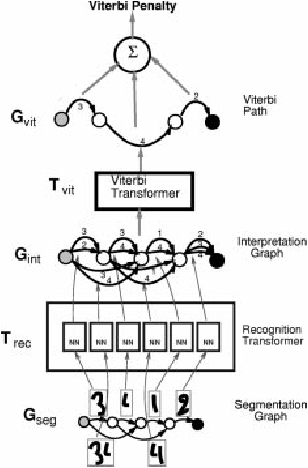
B. Recognition Transformer and Viterbi Transformer
A simple GTN to recognize character strings is shown in Fig. 17. It is composed of two GT’s called the recognition transformer and the Viterbi transformer . The goal of the recognition transformer is to generate a graph, called the interpretation graph or recognition graph , that contains all the possible interpretations for all the possible segmentations of the input. Each path in represents one possible interpretation of one particular segmentation of the input. The role of the Viterbi transformer is to extract the best interpretation from the interpretation graph.
The recognition transformer takes the segmentation graph as input, and applies the recognizer for single characters to the images associated with each of the arcs in the segmentation graph. The interpretation graph has almost the same structure as the segmentation graph, except that each arc is replaced by a set of arcs from and to the same node. In this set of arcs, there is one arc for each possible class for the image associated with the corresponding arc in . As shown in Fig. 18, to each arc is attached a class label, and the penalty that the image belongs to this class as produced by the recognizer. If the segmentor has computed penalties for the candidate segments, these penalties are combined with the penalties computed by the character recognizer to obtain the penalties on the arcs of the interpretation graph. Although combining penalties of different nature seems highly heuristic, the GTN training procedure will tune the penalties and take advantage of this combination anyway. Each path in the interpretation graph corresponds to a possible interpretation of the input word. The penalty of a particular interpretation for a particular segmentation is given by the sum of the arc penalties along the corresponding path in the interpretation graph. Computing the penalty of an interpretation independently of the segmentation requires to combine the penalties of all the paths with that interpretation. An appropriate rule for combining the penalties of parallel paths is given in Section VI-C.
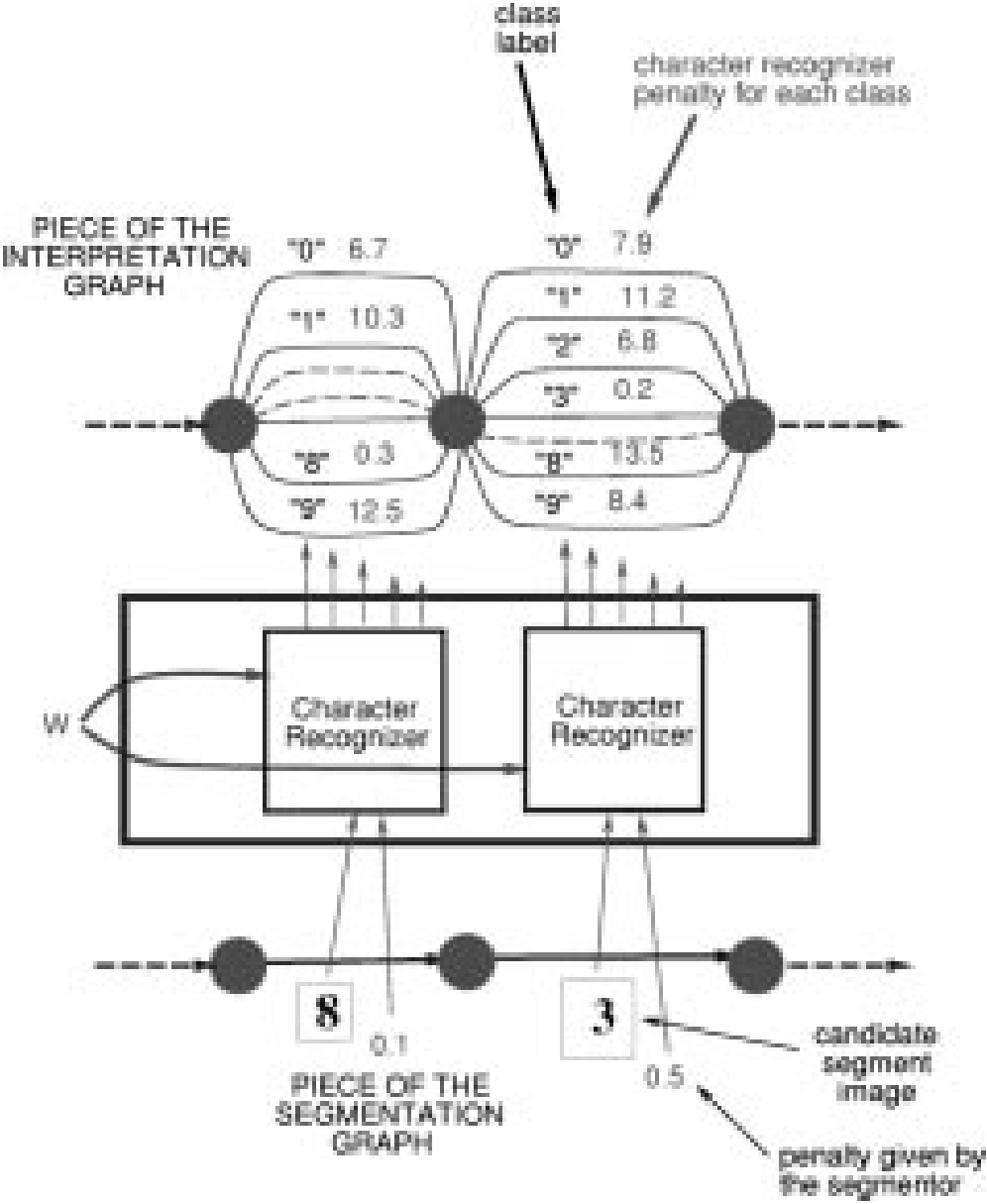
The Viterbi transformer produces a graph with a single path. This path is the path of least cumulated penalty in the Interpretation graph. The result of the recognition can be produced by reading off the labels of the arcs along the graph extracted by the Viterbi transformer. The Viterbi transformer owes its name to the famous Viterbi algorithm [70], an application of the principle of dynamic programming to find the shortest path in a graph efficiently. Let be the penalty associated to arc , with source node and destination node (note that there can be multiple arcs between two nodes). In the interpretation graph, arcs also have a label . The Viterbi algorithm proceeds as follows. Each node is associated with a cumulated Viterbi penalty . Those cumulated penalties are computed in any order that satisfies the partial order defined by the interpretation graph (which is directed and acyclic). The start node is initialized with the cumulated penalty . The other nodes cumulated penalties are computed recursively from the values of their parent nodes, through the upstream arcs
Furthermore, the value of for each node which minimizes the right-hand side is noted , the minimizing entering arc. When the end node is reached we obtain in , the total penalty of the path with the smallest total penalty. We call this penalty the Viterbi penalty, and this sequence of arcs and nodes the Viterbi path. To obtain the Viterbi path with nodes and arcs , we trace back these nodes and arcs as follows, starting with the end node, and recursively using the minimizing entering arc: , and until the start node is reached. The label sequence can then be read off the arcs of the Viterbi path.
VI GLOBAL TRAINING FOR GRAPH TRANSFORMER NETWORKS
Section V described the process of recognizing a string using HOS, assuming that the recognizer is trained so as to give low penalties for the correct class label of correctly segmented characters, high penalties for erroneous categories of correctly segmented characters, and high penalties for all categories for poorly formed characters. This section explains how to train the system at the string level to do the above without requiring manual labeling of character segments. This training will be performed with a GTN whose architecture is slightly different from the recognition architecture described in Section V.
In many applications, there is enough a priori knowledge about what is expected from each of the modules in order to train them separately. For example, with HOS one could individually label single-character images and train a character recognizer on them, but it might be difficult to obtain an appropriate set of noncharacter images to train the model to reject wrongly segmented candidates. Although separate training is simple, it requires additional supervision information that is often lacking or incomplete (the correct segmentation and the labels of incorrect candidate segments). Furthermore, it can be shown that separate training is suboptimal [67].
The following section describes four different gradient-based methods for training GTN-based handwriting recognizers at the string level: Viterbi training, discriminative Viterbi training, forward training, and discriminative forward training. The last one is a generalization to graph-based systems of the maximum a posteriori criterion introduced in Section II-C. Discriminative forward training is somewhat similar to the so-called maximum mutual information criterion used to train HMM in speech recognition. However, our rationale differs from the classical one. We make no recourse to a probabilistic interpretation but show that, within the gradient-based learning approach, discriminative training is a simple instance of the pervasive principle of error correcting learning.
Training methods for graph-based sequence recognition systems such as HMM’s have been extensively studied in the context of speech recognition [28]. Those methods require that the system be based on probabilistic generative models of the data, which provide normalized likelihoods over the space of possible input sequences. Popular HMM learning methods, such as the Baum–Welsh algorithm, rely on this normalization. The normalization cannot be preserved when nongenerative models such as NN’s are integrated into the system. Other techniques, such as discriminative training methods, must be used in this case. Several authors have proposed such methods to train NN/HMM speech recognizers at the word or sentence level [29], [67], [71]–[78].
Other globally trainable sequence recognition systems avoid the difficulties of statistical modeling by not resorting to graph-based techniques. The best example is recurrent NN’s (RNN’s). Unfortunately, despite early enthusiasm, the training of RNN’s with gradient-based techniques has proven very difficult in practice [79].
The GTN techniques presented below simplify and generalize the global training methods developed for speech recognition.
A. Viterbi Training
During recognition, we select the path in the interpretation graph that has the lowest penalty with the Viterbi algorithm. Ideally, we would like this path of lowest penalty to be associated with the correct label sequence as often as possible. An obvious loss function to minimize is therefore the average over the training set of the penalty of the path associated with the correct label sequence that has the lowest penalty. The goal of training will be to find the set of recognizer parameters (the weights, if the recognizer is an NN) that minimize the average penalty of this “correct” lowest penalty path. The gradient of this loss function can be computed by back propagation through the GTN architecture shown in Fig. 19. This training architecture is almost identical to the recognition architecture described in the previous section, except that an extra GT called a path selector is inserted between the interpretation graph and the Viterbi transformer. This transformer takes the interpretation graph and the desired label sequence as input. It extracts from the interpretation graph those paths that contain the correct (desired) label sequence. Its output graph is called the constrained interpretation graph (also known as forced alignment in the HMM literature) and contains all the paths that correspond to the correct label sequence. The constrained interpretation graph is then sent to the Viterbi transformer which produces a graph with a single path. This path is the “correct” path with the lowest penalty. Finally, a path scorer transformer takes and simply computes its cumulated penalty by adding up the penalties along the path. The output of this GTN is the loss function for the current pattern
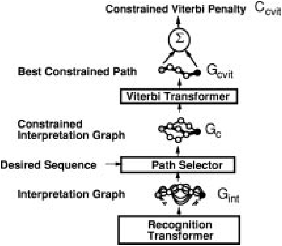
The only label information that is required by the above system is the sequence of desired character labels. No knowledge of the correct segmentation is required on the part of the supervisor, since it chooses among the segmentations in the interpretation graph the one that yields the lowest penalty.
The process of back propagating gradients through the Viterbi training GTN is now described. As explained in Section IV, the gradients must be propagated backward through all modules of the GTN in order to compute gradients in preceding modules and thereafter tune their parameters. Back propagating gradients through the path scorer is quite straightforward. The partial derivatives of the loss function with respect to the individual penalties on the constrained Viterbi path are equal to one, since the loss function is simply the sum of those penalties. Back propagating through the Viterbi Transformer is equally simple. The partial derivatives of with respect to the penalties on the arcs of the constrained graph are one for those arcs that appear in the constrained Viterbi path and zero for those that do not. Why is it legitimate to back propagate through an essentially discrete function such as the Viterbi transformer? The answer is that the Viterbi transformer is nothing more than a collection of min functions and adders put together. It was shown in Section IV that gradients can be back propagated through min functions without adverse effects. Back propagation through the path selector transformer is similar to back propagation through the Viterbi transformer. Arcs in that appear in have the same gradient as the corresponding arc in , i.e., one or zero, depending on whether the arc appear in . The other arcs, i.e., those that do not have an alter ego in because they do not contain the right label have a gradient of zero. During the forward propagation through the recognition transformer, one instance of the recognizer for single character was created for each arc in the segmentation graph. The state of recognizer instances was stored. Since each arc penalty in is produced by an individual output of a recognizer instance, we now have a gradient (one or zero) for each output of each instance of the recognizer. Recognizer outputs that have a nonzero gradient are part of the correct answer and will therefore have their value pushed down. The gradients present on the recognizer outputs can be back propagated through each recognizer instance. For each recognizer instance, we obtain a vector of partial derivatives of the loss function with respect to the recognizer instance parameters. All the recognizer instances share the same parameter vector, since they are merely clones of each other, therefore the full gradient of the loss function with respect to the recognizer’s parameter vector is simply the sum of the gradient vectors produced by each recognizer instance. Viterbi training, though formulated differently, is often use in HMM-based speech recognition systems [28]. Similar algorithms have been applied to speech recognition systems that integrate NN’s with time alignment [71], [72], [76] or hybrid neural-network/HMM systems [29], [74], [75].
While it seems simple and satisfying, this training architecture has a flaw that can potentially be fatal. The problem was already mentioned in Section II-C. If the recognizer is a simple NN with sigmoid output units, the minimum of the loss function is attained, not when the recognizer always gives the right answer, but when it ignores the input and sets its output to a constant vector with small values for all the components. This is known as the collapse problem. The collapse only occurs if the recognizer outputs can simultaneously take their minimum value. If, on the other hand, the recognizer’s output layer contains RBF units with fixed parameters, then there is no such trivial solution. This is due to the fact that a set of RBF with fixed distinct parameter vectors cannot simultaneously take their minimum value. In this case, the complete collapse described above does not occur. However, this does not totally prevent the occurrence of a milder collapse because the loss function still has a “flat spot” for a trivial solution with constant recognizer output. This flat spot is a saddle point, but it is attractive in almost all directions and is very difficult to get out of using gradient-based minimization procedures. If the parameters of the RBF’s are allowed to adapt, then the collapse problems reappear because the RBF centers can all converge to a single vector, and the underlying NN can learn to produce that vector and ignore the input. A different kind of collapse occurs if the width of the RBF’s are also allowed to adapt. The collapse only occurs if a trainable module such as an NN feeds the RBF’s. The collapse does not occur in HMM-based speech recognition systems because they are generative systems that produce normalized likelihoods for the input data (more on this later). Another way to avoid the collapse is to train the whole system with respect to a discriminative training criterion, such as maximizing the conditional probability of the correct interpretations (correct sequence of class labels) given the input image.
Another problem with Viterbi training is that the penalty of the answer cannot be used reliably as a measure of confidence because it does not take low-penalty (or high-scoring) competing answers into account.
B. Discriminative Viterbi Training
A modification of the training criterion can circumvent the collapse problem described above and at the same time produce more reliable confidence values. The idea is to not only minimize the cumulated penalty of the lowest penalty path with the correct interpretation, but also to somehow increase the penalty of competing and possibly incorrect paths that have a dangerously low penalty. This type of criterion is called discriminative because it plays the good answers against the bad ones. Discriminative training procedures can be seen as attempting to build appropriate separating surfaces between classes rather than to model individual classes independently of each other. For example, modeling the conditional distribution of the classes given the input image is more discriminative (focusing more on the classification surface) than having a separate generative model of the input data associated to each class (which, with class priors, yields the whole joint distribution of classes and inputs). This is because the conditional approach does not need to assume a particular form for the distribution of the input data.
One example of discriminative criterion is the difference between the penalty of the Viterbi path in the constrained graph, and the penalty of the Viterbi path in the (unconstrained) interpretation graph, i.e., the difference between the penalty of the best correct path and the penalty of the best path (correct or incorrect). The corresponding GTN training architecture is shown in Fig. 20. The left side of the diagram is identical to the GTN used for nondiscriminative Viterbi training. This loss function reduces the risk of collapse because it forces the recognizer to increases the penalty of wrongly recognized objects. Discriminative training can also be seen as another example of error correction procedure, which tends to minimize the difference between the desired output computed in the left half of the GTN in Fig. 20 and the actual output computed in the right half of Fig. 20.
Let the discriminative Viterbi loss function be denoted , and let us call the penalty of the Viterbi path in the constrained graph and the penalty of the Viterbi path in the unconstrained interpretation graph
is always positive since the constrained graph is a subset of the paths in the interpretation graph, and the Viterbi algorithm selects the path with the lowest total penalty. In the ideal case, the two paths and coincide, and is zero.
Back-propagating gradients through the discriminative Viterbi GTN adds some “negative” training to the previously described nondiscriminative training. Fig. 20 shows how the gradients are back propagated. The left half is identical to the nondiscriminative Viterbi training GTN, therefore the back propagation is identical. The gradients back propagated through the right half of the GTN are multiplied by , since contributes to the loss with a negative sign. Otherwise the process is similar to the left half. The gradients on arcs of get positive contributions from the left half and negative contributions from the right half. The two contributions must be added since the penalties on arcs are sent to the two halves through a “Y” connection in the forward pass. Arcs in that appear neither in nor in have a gradient of zero. They do not contribute to the cost. Arcs that appear in both and also have zero gradient. The contribution from the right half cancels the contribution from the left half. In other words, when an arc is rightfully part of the answer there is no gradient. If an arc appears in but not in , the gradient is . The arc should have had a lower penalty to make it to . If an arc is in but not in , the gradient is . The arc had a low penalty, but it should have had a higher penalty since it is not part of the desired answer.
Variations of this technique have been used for the speech recognition. Driancourt and Bottou [76] used a version of it where the loss function is saturated to a fixed value. This can be seen as a generalization of the Learning Vector Quantization 2 (LVQ-2) loss function [80]. Other variations of this method use not only the Viterbi path but the K-best paths. The discriminative Viterbi algorithm does not have the flaws of the nondiscriminative version, but there are problems nonetheless. The main problem is that the criterion does not build a margin between the classes. The gradient is zero as soon as the penalty of the constrained Viterbi path is equal to that of the Viterbi path. It would be desirable to push up the penalties of the wrong paths when they are dangerously close to the good one. The following section presents a solution to this problem.
C. Forward Scoring and Forward Training
While the penalty of the Viterbi path is perfectly appropriate for the purpose of recognition it gives only a partial picture of the situation. Imagine the lowest penalty paths corresponding to several different segmentations produced the same answer (the same label sequence). Then it could be argued that the overall penalty for the interpretation should be smaller than the penalty obtained when only one path produced that interpretation, because multiple paths with identical label sequences are more evidence that the label sequence is correct. Several rules can be used compute the penalty associated to a graph that contains several parallel paths. We use a combination rule borrowed from a probabilistic interpretation of the penalties as negative log posteriors. In a probabilistic framework, the posterior probability for the interpretation should be the sum of the posteriors for all the paths that produce that interpretation.
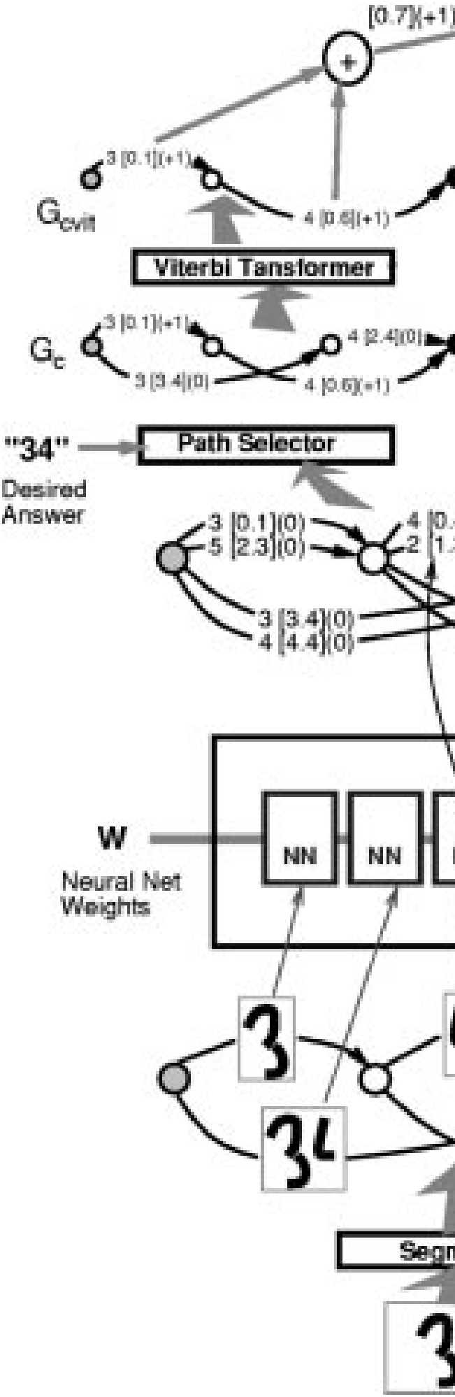
Translated in terms of penalties, the penalty of an interpretation should be the negative logarithm of the sum of the negative exponentials of the penalties of the individual paths. The overall penalty will be smaller than all the penalties of the individual paths.
Given an interpretation, there is a well-known method, called the forward algorithm for computing the above quantity efficiently [28]. The penalty computed with this procedure for a particular interpretation is called the forward penalty. Consider again the concept of constrained
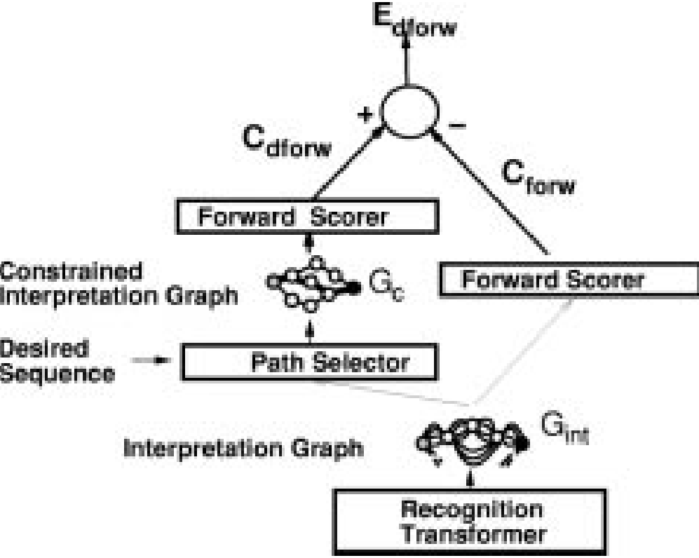
the forward penalty of the complete interpretation graph
is always positive since the constrained graph is a subset of the paths in the interpretation graph, and the forward penalty of a graph is always larger than the forward penalty of a subgraph of this graph. In the ideal case, the penalties of incorrect paths are infinitely large, therefore the two penalties coincide and is zero. Readers familiar with the Boltzmann machine connectionist model might recognize the constrained and unconstrained graphs as analogous to the “clamped” (constrained by the observed values of the output variable) and “free” (unconstrained) phases of the Boltzmann machine algorithm [13].
Back propagating derivatives through the discriminative forward GTN distributes gradients more evenly than in the Viterbi case. Derivatives are back propagated through the left half of the GTN in Fig. 21 down to the interpretation graph. Derivatives are negated and back propagated through the right-half, and the result for each arc is added to the contribution from the left half. Each arc in now has a derivative. Arcs that are part of a correct path have a positive derivative. This derivative is very large if an incorrect path has a lower penalty than all the correct paths. Similarly, the derivatives with respect to arcs that are part of a low-penalty incorrect path have a large negative derivative. On the other hand, if the penalty of a path associated with the correct interpretation is much smaller than all other paths, the loss function is very close to zero and almost no gradient is back propagated. The training therefore concentrates on examples of images which yield a classification error, and furthermore, it concentrates on the pieces of the image which cause that error. Discriminative forward training is an elegant and efficient way of solving the infamous credit assignment problem for learning machines that manipulate “dynamic” data structures such as graphs. More generally, the same idea can be used in all situations where a learning machine must choose between discrete alternative interpretations.
As previously, the derivatives on the interpretation graph penalties can then be back propagated into the character recognizer instances. Back propagation through the character recognizer gives derivatives on its parameters. All the gradient contributions for the different candidate segments are added up to obtain the total gradient associated to one pair (input image, correct label sequence), that is, one example in the training set. A step of stochastic gradient descent can then be applied to update the parameters.
E. Remarks on Discriminative Training
In the above discussion, the global training criterion was given a probabilistic interpretation, but the individual penalties on the arcs of the graphs were not. There are good reasons for that. For example, if some penalties are associated to the different class labels, they would: 1) have to sum to one (class posteriors) or 2) integrate to one over the input domain (likelihoods).
Let us first discuss the first case (class posteriors normalization). This local normalization of penalties may eliminate information that is important for locally rejecting all the classes [82], e.g., when a piece of image does not correspond to a valid character class because some of the segmentation candidates may be wrong. Although an explicit “garbage class” can be introduced in a probabilistic framework to address that question, some problems remain because it is difficult to characterize such a class probabilistically and to train a system in this way (it would require a density model of unseen or unlabeled samples).
The probabilistic interpretation of individual variables plays an important role in the Baum–Welsh algorithm in combination with the expectation-maximization (EM) procedure. Unfortunately, those methods cannot be applied to discriminative training criteria, and one is reduced to using gradient-based methods. Enforcing the normalization of the probabilistic quantities while performing gradient-based learning is complex, inefficient, time consuming, and creates ill-conditioning of the loss-function.
Following [82], we therefore prefer to postpone normalization as far as possible (in fact, until the final decision stage of the system). Without normalization, the quantities manipulated in the system do not have a direct probabilistic interpretation.
Let us now discuss the second case (using a generative model of the input). Generative models build the boundary indirectly by first building an independent density model for each class and then performing classification decisions on the basis of these models. This is not a discriminative approach in that it does not focus on the ultimate goal of learning, which in this case is to learn the classification decision surface. Theoretical arguments [6], [7] suggest that estimating input densities when the real goal is to obtain a discriminant function for classification is a suboptimal strategy. In theory, the problem of estimating densities in high-dimensional spaces is much more ill posed than finding decision boundaries.
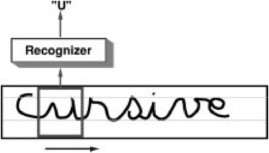
Even though the internal variables of the system do not have a direct probabilistic interpretation, the overall system can still be viewed as producing posterior probabilities for the classes. In fact, assuming that a particular label sequence is given as the “desired sequence” to the GTN in Fig. 21, the exponential of minus can be interpreted as an estimate of the posterior probability of that label sequence given the input. The sum of those posteriors for all the possible label sequences is one. Another approach would consists of directly minimizing an approximation of the number of misclassifications [83], [76]. We prefer to use the discriminative forward loss function because it causes less numerical problems during the optimization. We will see in Section X-C that this is a good way to obtain scores on which to base a rejection strategy. The important point being made here is that one is free to choose any parameterization deemed appropriate for a classification model. The fact that a particular parameterization uses internal variables with no clear probabilistic interpretation does not make the model any less legitimate than models that manipulate normalized quantities.
An important advantage of global and discriminative training is that learning focuses on the most important errors, and the system learns to integrate the ambiguities from the segmentation algorithm with the ambiguities of the character recognizer. In Section IX we present experimental results with an online handwriting recognition system that confirm the advantages of using global training versus separate training. Experiments in speech recognition with hybrids of NN’s and HMM’s also showed marked improvements brought by global training [29], [67], [77], [84].
VII MULTIPLE OBJECT RECOGNITION: SPACE DISPLACEMENT NEURAL NETWORK
There is a simple alternative to explicitly segmenting images of character strings using heuristics. The idea is to sweep a recognizer at all possible locations across a normalized image of the entire word or string as shown in Fig. 22. With this technique, no segmentation heuristics are required since the system essentially examines all the possible segmentations of the input. However, there are problems with this approach. First, the method is in general quite expensive. The recognizer must be applied at every possible location on the input, or at least at a large enough subset of locations so that misalignments of characters in the field of view of the recognizers are small enough to have no effect on the error rate. Second, when the recognizer is centered on a character to be recognized, the neighbors of the center character will be present in the field of view of the recognizer, possibly touching the center character. Therefore the recognizer must be able to correctly recognize the character in the center of its input field, even if neighboring characters are very close to or touching the central character. Third, a word or character string cannot be perfectly size-normalized. Individual characters within a string may have widely varying sizes and baseline positions. Therefore the recognizer must be very robust to shifts and size variations.
These three problems are elegantly circumvented if a convolutional network is replicated over the input field. First of all, as shown in Section III, convolutional NN’s are very robust to shifts and scale variations of the input image, as well as to noise and extraneous marks in the input. These properties take care of the latter two problems mentioned in the previous paragraph. Second, convolutional networks provide a drastic saving in computational requirement when replicated over large input fields. A replicated convolutional network, also called an SDNN [27], is shown in Fig. 23. While scanning a recognizer can be prohibitively expensive in general, convolutional networks can be scanned or replicated very efficiently over large, variable-size input fields. Consider one instance of a convolutional net and its alter ego at a nearby location. Because of the convolutional nature of the network, units in the two instances that look at identical locations on the input have identical outputs, therefore their states do not need to be computed twice. Only a thin “slice” of new states that are not shared by the two network instances needs to be recomputed. When all the slices are put together, the result is simply a larger convolutional network whose structure is identical to the original network, except that the feature maps are larger in the horizontal dimension. In other words, replicating a convolutional network can be done simply by increasing the size of the fields over which the convolutions are performed and by replicating the output layer accordingly. The output layer effectively becomes a convolutional layer. An output whose receptive field is centered on an elementary object will produce the class of this object, while an in-between output may indicate no character or contain rubbish. The outputs can be interpreted as evidences for the presence of objects at all possible positions in the input field.
The SDNN architecture seems particularly attractive for recognizing cursive handwriting where no reliable segmentation heuristic exists. Although the idea of SDNN is quite old and very attractive in its simplicity, it has not generated wide interest until recently because, as stated above, it puts enormous demands on the recognizer [26], [27]. In speech recognition, where the recognizer is at least one order of magnitude smaller, replicated convolutional networks are easier to implement, for instance in Haffner’s multistate TDNN model [78], [85].
A. Interpreting the Output of an SDNN with a GTN
The output of an SDNN is a sequence of vectors which encode the likelihoods, penalties, or scores of finding character of a particular class label at the corresponding location in the input. A postprocessor is required to pull out the best possible label sequence from this vector sequence. An example of SDNN output is shown in Fig. 25. Very often, individual characters are spotted by several neighboring instances of the recognizer, a consequence of the robustness of the recognizer to horizontal translations. Also quite often, characters are erroneously detected by recognizer instances that see only a piece of a character. For example a recognizer instance that only sees the right third of a “4” might output the label 1. How can we eliminate those extraneous characters from the output sequence and pull out the best interpretation? This can be done using a new type of GT with two input graphs as shown in Fig. 24. The sequence of vectors produced by the SDNN is first coded into a linear graph with multiple arcs between pairs of successive nodes. Each arc between a particular pair of nodes contains the label of one of the possible categories, together with the penalty produced by the SDNN for that class label at that location. This graph is called the SDNN output graph. The second input graph to the transformer is a grammar transducer, more specifically a finite-state transducer [86], that encodes the relationship between input strings of class labels and corresponding output strings of recognized characters. The transducer is a weighted finite state machine (a graph) where each arc contains a pair of labels and possibly a penalty. Like a finite-state machine, a transducer is in a state and follows an arc to a new state when an observed input symbol matches the first symbol in the symbol pair attached to the arc. At this point the transducer emits the second symbol in the pair together with a penalty that combines the penalty of the input symbol and the penalty of the arc. A transducer therefore transforms a weighted symbol sequence into another weighted symbol sequence. The GT shown in Fig. 24 performs a composition between the recognition graph and the grammar transducer. This operation takes every possible sequence corresponding to every possible path in the recognition graph and matches them with the paths in the grammar transducer. The composition produces the interpretation graph, which contains a path for each corresponding output label sequence. This composition operation may seem combinatorially intractable, but it turns out there exists an efficient algorithm for it described in more details in Section VIII.
B. Experiments with SDNN
In a series of experiments, LeNet-5 was trained with the goal of being replicated so as to recognize multiple characters without segmentations. The data were generated from the previously described MNIST set as follows. Training images were composed of a central character, flanked by two side characters picked at random in the training set. The separation between the bounding boxes of the characters were chosen at random between −1 and 4 pixels. In other instances, no central character was present, in which case the desired output of the network was the blank space class. In addition, training images were degraded with 10% salt and pepper noise (random pixel inversions).
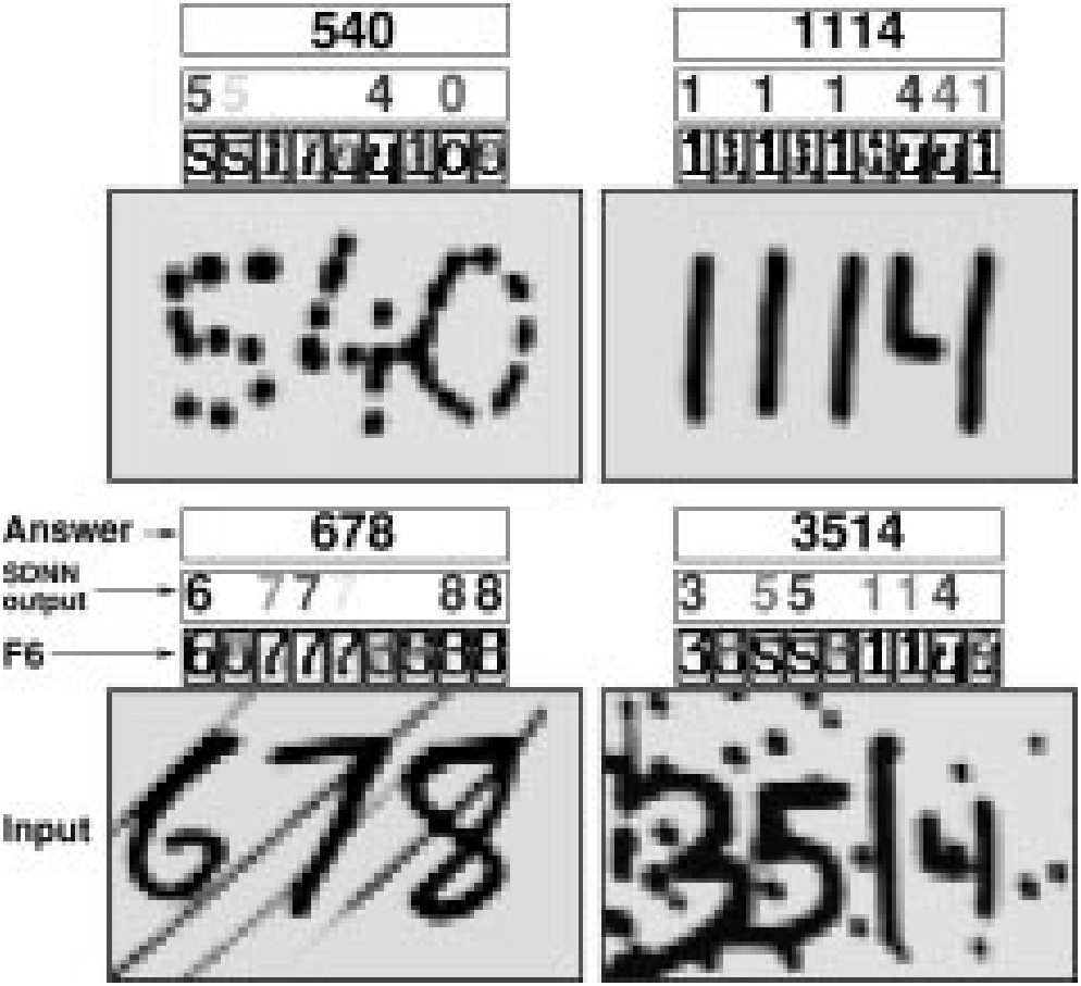
Figs. 25 and 26 show a few examples of successful recognitions of multiple characters by the LeNet-5 SDNN. Standard techniques based on HOS would fail miserably on many of those examples. As can be seen on these examples, the network exhibits striking invariance and noise resistance properties. While some authors have argued that invariance requires more sophisticated models than feedforward NN’s [87], LeNet-5 exhibits these properties to a large extent.
Similarly, it has been suggested that accurate recognition of multiple overlapping objects require explicit mechanisms that would solve the so-called feature binding problem [87]. As can be seen on Figs. 25 and 26, the network is able to tell the characters apart even when they are closely intertwined, a task that would be impossible to achieve with the more classical HOS technique. The SDNN is also able to correctly group disconnected pieces of ink that form characters. Good examples of that are shown in the upper half of Fig. 26. In the top left example, the 4 and the 0 are more connected to each other than they are connected with themselves, yet the system correctly identifies the 4 and the 0 as separate objects. The top right example is interesting for several reasons. First the system correctly identifies the three individual ones. Second, the left half and right half of disconnected 4 are correctly grouped, even though no geometrical information could decide to associate the left half to the vertical bar on its left or on its right. The right half of the 4 does cause the appearance of an erroneous one on the SDNN output, but this one is removed by the character model transducer which prevents characters from appearing on contiguous outputs.
Another important advantage of SDNN is the ease with which they can be implemented on parallel hardware. Specialized analog/digital chips have been designed and used in character recognition, and in image preprocessing applications [88]. However the rapid progress of conventional processor technology with reduced-precision vector arithmetic instructions (such as Intel’s MMX) make the success of specialized hardware hypothetical at best.3
C. Global Training of SDNN
In the above experiments, the string images were artificially generated from individual character. The advantage is that we know in advance the location and the label of the important character. With real training data, the correct sequence of labels for a string is generally available, but the precise locations of each corresponding character in the input image are unknown.
In the experiments described in the previous section, the best interpretation was extracted from the SDNN output using a very simple GT. Global training of an SDNN can be performed by back propagating gradients through such GT’s arranged in architectures similar to the ones described in Section VI.
This is somewhat equivalent to modeling the output of an SDNN with an HMM. Globally trained, variable-size TDNN/HMM hybrids have been used for speech recognition and online handwriting recognition [67], [77], [89], [90]. SDNN’s have been used in combination with HMM’s or other elastic matching methods for handwritten word recognition [91], [92].
Fig. 27 shows the GT architecture for training an SDNN/HMM hybrid with the discriminative forward criterion. The top part is comparable to the top part of Fig. 21. On the right side the composition of the recognition graph with the grammar gives the interpretation graph with all the possible legal interpretations. On the left side the composition is performed with a grammar that only contains paths with the desired sequence of labels. This has a somewhat similar function to the path selector used in the previous section. Like in Section VI-D, the loss function is the difference between the forward score obtained from the left half and the forward score obtained from the right half. To back propagate through the composition transformer, we need to keep a record of which arc in the recognition graph originated which arcs in the interpretation graph. The derivative with respect to an arc in the recognition graph is equal to the sum of the derivatives with respect to all the arcs in the interpretation graph that originated from it. Derivative can also be computed for the penalties on the grammar graph, allowing to learn them as well. As in the previous example, a discriminative criterion must
3 Short video clips of the LeNet-5 SDNN are available WWW: http://www.research.att.com/˜yann/ocr.
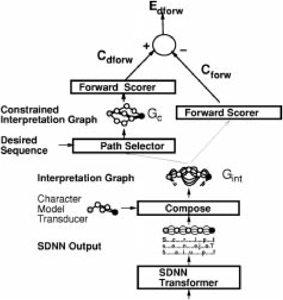
be used, because using a nondiscriminative criterion could result in a collapse effect if the network’s output RBF are adaptive. The above training procedure can be equivalently formulated in term of HMM. Early experiments in zip code recognition [91], and more recent experiments in online handwriting recognition [38] have demonstrated the idea of globally trained SDNN/HMM hybrids. SDNN is an extremely promising and attractive technique for OCR, but so far it has not yielded better results than HOS. We hope that these results will improve as more experience is gained with these models.
D. Object Detection and Spotting with SDNN
An interesting application of SDNN’s is object detection and spotting. The invariance properties of convolutional networks, combined with the efficiency with which they can be replicated over large fields, suggests that they can be used for “brute force” object spotting and detection in large images. The main idea is to train a single convolutional network to distinguish images of the object of interest from images present in the background. In utilization mode, the network is replicated so as to cover the entire image to be analyzed, thereby forming a 2-D SDNN. The output of the SDNN is a 2-D plane in which activated units indicate the presence of the object of interest in the corresponding receptive field. Since the sizes of the objects to be detected within the image are unknown, the image can be presented to the network at multiple resolutions, and the results at multiple resolutions combined. The idea has been applied to face location [93], address block location on envelopes [94], and hand tracking in video [95].
To illustrate the method, we will consider the case of face detection in images as described in [93]. First, images containing faces at various scales are collected. Those images are filtered through a zero-mean Laplacian filter so as to remove variations in global illumination and low spatial frequency illumination gradients. Then, training samples of faces and nonfaces are manually extracted from those images. The face subimages are then size normalized so that the height of the entire face is approximately 20 pixels while keeping fairly large variations (within a factor of two). The scale of background subimages are picked at random. A single convolutional network is trained on those samples to classify face subimages from nonface subimages.
When a scene image is to be analyzed, it is first filtered through the Laplacian filter and subsampled at powers-of-two resolutions. The network is replicated over each of multiple resolution images. A simple voting technique is used to combine the results from multiple resolutions.
A 2-D version of the global training method described in the previous section can be used to alleviate the need to manually locate faces when building the training sample [93]. Each possible location is seen as an alternative interpretation, i.e., one of several parallel arcs in a simple graph that only contains a start node and an end node.
Other authors have used NN’s or other classifiers such as SVM’s for face detection with great success [96], [97]. Their systems are very similar to the one described above, including the idea of presenting the image to the network at multiple scales. But since those systems do not use convolutional networks, they cannot take advantage of the speedup described here, and they have to rely on other techniques, such as prefiltering and real-time tracking, to keep the computational requirement within reasonable limits. In addition, because those classifiers are much less invariant to scale variations than convolutional networks, it is necessary to multiply the number of scales at which the images are presented to the classifier.
VIII Graph Transformer Networks and Transducers
In Section IV, GTN’s were introduced as a generalization of multilayer, multimodule networks where the state information is represented as graphs instead of fixed-size vectors. This section reinterprets the GTN’s in the framework of generalized transduction and proposes a powerful graph composition algorithm.
A. Previous Work
Numerous authors in speech recognition have used gradient-based learning methods that integrate graph-based statistical models (notably HMM’s) with acoustic recognition modules, mainly Gaussian mixture models, but also NN’s [67], [78], [98], [99]. Similar ideas have been applied to handwriting recognition (see [38] for a review). However, there has been no proposal for a systematic approach to multilayer graph-based trainable systems. The idea of transforming graphs into other graphs has received considerable attention in computer science through the concept of weighted finite-state transducers [86]. Transducers have been applied to speech recognition [100] and language translation [101], and proposals have been made for handwriting recognition [102]. This line of work has been mainly focused on efficient search algorithms [103] and on the algebraic aspects of combining transducers and graphs (called acceptors in this context), but very little effort has been devoted to building globally trainable systems out of transducers. What is proposed in the following sections is a systematic approach to automatic training in graph-manipulating systems. A different approach to graph-based trainable systems, called input–output HMM, was proposed in [104] and [105].
B. Standard Transduction
In the established framework of finite-state transducers [86], discrete symbols are attached to arcs in the graphs. Acceptor graphs have a single symbol attached to each arc whereas transducer graphs have two symbols (an input symbol and an output symbol). A special null symbol is absorbed by any other symbol (when concatenating symbols to build a symbol sequence). Weighted transducers and acceptors also have a scalar quantity attached to each arc. In this framework, the composition operation takes as input an acceptor graph and a transducer graph and builds an output acceptor graph. Each path in this output graph (with symbol sequence ) corresponds to one path (with symbol sequence ) in the input acceptor graph and one path and a corresponding pair of input–output sequences () in the transducer graph. The weights on the arcs of the output graph are obtained by adding the weights from the matching arcs in the input acceptor and transducer graphs. In the rest of the paper, we will call this graph composition operation using transducers the (standard) transduction operation.
A simple example of transduction is shown in Fig. 28. In this simple example, the input and output symbols on the transducer arcs are always identical. This type of transducer graph is called a grammar graph. To better understand the transduction operation, imagine two tokens sitting each on the start nodes of the input acceptor graph and the transducer graph. The tokens can freely follow any arc labeled with a null input symbol. A token can follow an arc labeled with a nonnull input symbol if the other token also follows an arc labeled with the same input symbol. We have an acceptable trajectory when both tokens reach the end nodes of their graphs (i.e., the tokens have reached the terminal configuration). This trajectory represents a sequence of input symbols that complies with both the acceptor and the transducer. We can then collect the corresponding sequence of output symbols along the trajectory of the transducer token. The above procedure produces a tree, but a simple technique described in Section VIII-C can be used to avoid generating multiple copies of certain subgraphs by detecting when a particular output state has already been seen.
The transduction operation can be performed very efficiently [106], but presents complex bookkeeping problems concerning the handling of all combinations of null and nonnull symbols. If the weights are interpreted as probabilities (normalized appropriately) then an acceptor graph represents a probability distribution over the language defined by the set of label sequences associated to all possible paths (from the start to the end node) in the graph.
An example of application of the transduction operation is the incorporation of linguistic constraints (a lexicon or a grammar) when recognizing words or other character strings. The recognition transformer produces the recognition graph (an acceptor graph) by applying the NN recognizer to each candidate segment. This acceptor graph is composed with a transducer graph for the grammar. The grammar transducer contains a path for each legal sequence of symbol, possibly augmented with penalties to indicate the relative likelihoods of the possible sequences. The arcs contain identical input and output symbols. Another example of transduction was mentioned in Section V: the path selector used in the HOS training GTN is implementable by a composition. The transducer graph is linear graph which contains the correct label sequence. The composition of the interpretation graph with this linear graph yields the constrained graph.
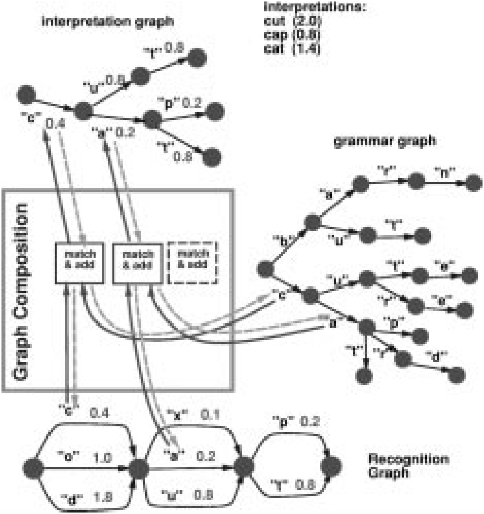
C. Generalized Transduction
If the data structures associated to each arc took only a finite number of values, composing the input graph and an appropriate transducer would be a sound solution. For our applications however, the data structures attached to the arcs of the graphs may be vectors, images or other high-dimensional objects that are not readily enumerated. We present a new composition operation that solves this problem.
Instead of only handling graphs with discrete symbols and penalties on the arcs, we are interested in considering graphs whose arcs may carry complex data structures, including continuous-valued data structures such as vectors and images. Composing such graphs requires additional information.
- When examining a pair of arcs (one from each input graph), we need a criterion to decide whether to create corresponding arc(s) and node(s) in the output graph, based on the information attached to the input arcs. We can decide to build an arc, several arcs, or an entire subgraph with several nodes and arcs.
- When that criterion is met, we must build the corresponding arc(s) and node(s) in the output graph and compute the information attached to the newly created arc(s) as a function that the information attached to the input arcs.
These functions are encapsulated in an object called a composition transformer. An instance of composition transformer implements the following three methods:
- check (arc1, arc2) compares the data structures pointed to by arcs arc1 (from the first graph) and arc2 (from the second graph) and returns a boolean indicating whether corresponding arc(s) should be created in the output graph;
- fprop (ngraph, upnode, downnode, arc1, arc2) is called when check (arc1, arc2) returns true; this method creates new arcs and nodes between nodes upnode and downnode in the output graph ngraph, and computes the information attached to these newly created arcs as a function of the attached information of the input arcs arc1 and arc2;
- bprop (ngraph, upnode, downnode, arc1, arc2) is called during training in order to propagate gradient information from the output subgraph between upnode and downnode into the data structures on the arc1 and arc2, as well as with respect to the parameters that were used in the fprop call with the same arguments; this method assumes that the function used by fprop to compute the values attached to its output arcs is differentiable.
The check method can be seen as constructing a dynamic architecture of functional dependencies, while the fprop method performs a forward propagation through that architecture to compute the numerical information attached to the arcs. The bprop method performs a backward propagation through the same architecture to compute the partial derivatives of the loss function with respect to the information attached to the arcs. This is illustrated in Fig. 28.
Fig. 29 shows a simplified generalized graph composition algorithm. This simplified algorithm does not handle null transitions, and it does not check whether the tokens
Function generalized_composition(PGRAPH graph1, PGRAPH graph2, PTRANS trans) { // Create new graph PGRAPH ngraph = new_graph()
// Create map between token positions // and nodes of the new graph PNODE map[PNODE,PNODE] = new_empty_map() map[endnode(graph1), endnode(graph2)] = endnode(newgraph)
// Recursive subroutine for simulating tokens Function simtokens(PNODE node1, PNODE node2) Returns PNODE { PNODE currentnode = map[node1, node2] // Check if already visited If (currentnode == nil) // Record new configuration currentnode = ngraph->create_node() map[node1, node2] = currentnode // Enumerate the possible non-null // joint token transitions For ARC arc1 in down_arcs(node1) For ARC arc2 in down_arcs(node2) If (trans->check(arc1, arc2)) PNODE newnode = simtokens(down_node(arc1), down_node(arc2)) trans->fprop(ngraph, currentnode, newnode, arc1, arc2) // Return node in composed graph Return currentnode }
// Perform token simulation simtokens(startnode(graph1), startnode(graph2)) Delete map Return ngraph } trajectory is acceptable (i.e., both tokens simultaneously reach the end nodes of their graphs). The management of null transitions is a straightforward modification of the token simulation function. Before enumerating the possible nonnull joint token transitions, we loop on the possible null transitions of each token, recursively call the token simulation function, and finally call the method fprop. The safest way for identifying acceptable trajectories consists of running a preliminary pass for identifying the token configurations from which we can reach the terminal configuration (i.e., both tokens on the end nodes). This is easily achieved by enumerating the trajectories in the opposite direction. We start on the end nodes and follow the arcs upstream. During the main pass, we only build the nodes that allow the tokens to reach the terminal configuration.
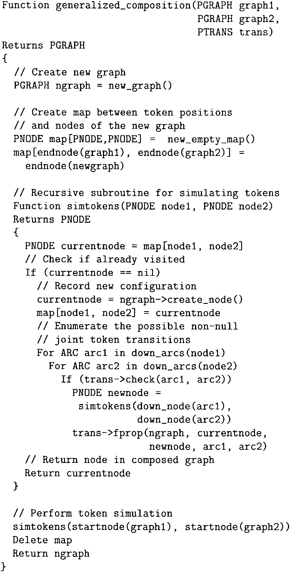
Graph composition using transducers (i.e., standard transduction) is easily and efficiently implemented as a generalized transduction. The method check simply tests the equality of the input symbols on the two arcs, and the method fprop creates a single arc whose symbol is the output symbol on the transducer’s arc.
The composition between pairs of graphs is particularly useful for incorporating linguistic constraints in a handwriting recognizer. Examples of its use are given in the online handwriting recognition system described in Section IX (and in the check reading system described in Section X).
In the rest of the paper, the term composition transformer will denote a GT based on the generalized transductions of multiple graphs. The concept of generalized transduction is a very general one. In fact, many of the GT’s described earlier in this paper, such as the segmenter and the recognizer, can be formulated in terms of generalized transduction. In this case, the generalized transduction does not take two input graphs but a single input graph. The method fprop of the transformer may create several arcs or even a complete subgraph for each arc of the initial graph. In fact the pair check, fprop itself can be seen as procedurally defining a transducer.
In addition, it can be shown that the generalized transduction of a single graph is theoretically equivalent to the standard composition of this graph with a particular transducer graph. However, implementing the operation this way may be very inefficient since the transducer can be very complicated.
In practice, the graph produced by a generalized transduction is represented procedurally in order to avoid building the whole output graph (which may be huge when for example the interpretation graph is composed with the grammar graph). We only instantiate the nodes which are visited by the search algorithm during recognition (e.g., Viterbi). This strategy propagates the benefits of pruning algorithms (e.g., beam search) in all the GTN’s.
D. Notes on the Graph Structures
Section VI discussed the idea of global training by back-propagating gradient through simple GT’s. The bprop method is the basis of the back-propagation algorithm for generic GT’s. A generalized composition transformer can be seen as dynamically establishing functional relationships between the numerical quantities on the input and output arcs. Once the check function has decided that a relationship should be established, the fprop function implements the numerical relationship. The check function establishes the structure of the ephemeral network inside the composition transformer.
Since fprop is assumed to be differentiable, gradients can be back propagated through that structure. Most parameters affect the scores stored on the arcs of the successive graphs of the system. A few threshold parameters may determine whether an arc appears or not in the graph. Since nonexisting arcs are equivalent to arcs with very large penalties, we only consider the case of parameters affecting the penalties.
In the kind of systems we have discussed until now (and the application described in Section X), much of the knowledge about the structure of the graph that is produced by a GT is determined by the nature of the GT, but it may also depend on the value of the parameters and on the input. It may also be interesting to consider GT modules which attempt to learn the structure of the output graph. This might be considered a combinatorial problem and not amenable to gradient-based learning, but a solution to this problem is to generate a large graph that contains the graph candidates as subgraphs, and then select the appropriate subgraph.
E. GTN and HMM’s
GTN’s can be seen as a generalization and an extension of HMM’s. On the one hand, the probabilistic interpretation can be either kept (with penalties being log-probabilities), pushed to the final decision stage (with the difference of the constrained forward penalty and the unconstrained forward penalty being interpreted as negative log-probabilities of label sequences), or dropped altogether (the network just represents a decision surface for label sequences in input space). On the other hand, GTN’s extend HMM’s by allowing to combine in a well-principled framework multiple levels of processing, or multiple models (e.g., Pereira et al. have been using the transducer framework for stacking HMM’s representing different levels of processing in automatic speech recognition [86]).
Unfolding an HMM in time yields a graph that is very similar to our interpretation graph (at the final stage of processing of the GTN, before Viterbi recognition). It has nodes associated to each time step and state in the model. The penalty for an arc from to then corresponds to the negative log-probability of emitting observed data at position and going from state to state in the time interval . With this probabilistic interpretation, the forward penalty is the negative logarithm of the likelihood of whole observed data sequence (given the model).
In Section VI we mentioned that the collapsing phenomenon can occur when nondiscriminative loss functions are used to train NN’s/HMM hybrid systems. With classical HMM’s with fixed preprocessing, this problem does not occur because the parameters of the emission and transition probability models are forced to satisfy certain probabilistic constraints: the sum or the integral of the probabilities of a random variable over its possible values must be one. Therefore, when the probability of certain events is increased, the probability of other events must automatically be decreased. On the other hand, if the probabilistic assumptions in an HMM (or other probabilistic model) are not realistic, discriminative training, discussed in Section VI, can improve performance as this has been clearly shown for speech recognition systems [48]–[50], [107], [108].
The input–output HMM (IOHMM) [105], [109] is strongly related to GT’s. Viewed as a probabilistic model, an IOHMM represents the conditional distribution of output sequences given input sequences (of the same or a different length). It is parameterized from an emission probability module and a transition probability module. The emission probability module computes the conditional emission probability of an output variable (given an input value and the value of discrete “state” variable). The transition probability module computes conditional transition probabilities of a change in the value of the “state” variable, given the input value. Viewed as a GT, it assigns an output graph (representing a probability distribution over the sequences of the output variable) to each path in the input graph. All these output graphs have the same structure, and the penalties on their arcs are simply added in order to obtain the complete output graph. The input values of the emission and transition modules are read off the data structure on the input arcs of the IOHMM GT. In practice, the output graph may be very large, and needs not be completely instantiated (i.e., it is pruned: only the low penalty paths are created).
IX AN ON-LINE HANDWRITING RECOGNITION SYSTEM
Natural handwriting is often a mixture of different “styles,” i.e., lower case printed, upper case, and cursive. A reliable recognizer for such handwriting would greatly improve interaction with pen-based devices, but its implementation presents new technical challenges. Characters taken in isolation can be very ambiguous, but considerable information is available from the context of the whole word. We have built a word recognition system for pen-based devices based on four main modules: 1) a preprocessor that normalizes a word, or word group, by fitting a geometrical model to the word structure; 2) a module that produces an “annotated image” from the normalized pen trajectory; 3) a replicated convolutional NN that spots and recognizes characters; and 4) a GTN that interprets the networks output by taking word-level constraints into account. The network and the GTN are jointly trained to minimize an error measure defined at the word level.
In this work, we have compared a system based on SDNN’s (such as described in Section VII), and a system based on HOS (such as described in Section V). Because of the sequential nature of the information in the pen trajectory (which reveals more information than the purely optical input from in image), HOS can be very efficient in proposing candidate character cuts, especially for noncursive script.
A. Preprocessing
Input normalization reduces intracharacter variability, thereby simplifying character recognition. We have used a word normalization scheme [92] based on fitting a geometrical model of the word structure. Our model has four “flexible” lines representing respectively the ascenders line, the core line, the base line, and the descenders line. The lines are fitted to local minima or maxima of the pen trajectory. The parameters of the lines are estimated with a modified version of the EM algorithm to maximize the joint probability of observed points and parameter values, using a prior on parameters that prevents the lines from collapsing on each other.
The recognition of handwritten characters from a pen trajectory on a digitizing surface is often done in the time domain [44], [110], [111]. Typically, trajectories are normalized and local geometrical or dynamical features are extracted. The recognition may then be performed using curve matching [110], or other classification techniques such as TDNN’s [44], [111]. While these representations have several advantages, their dependence on stroke ordering and individual writing styles makes them difficult to use in high accuracy, writer independent systems that integrate the segmentation with the recognition.
Since the intent of the writer is to produce a legible image, it seems natural to preserve as much of the pictorial nature of the signal as possible, while at the same time exploit the sequential information in the trajectory. For this purpose we have designed a representation scheme called AMAP [38], where pen trajectories are represented by low-resolution images in which each picture element contains information about the local properties of the trajectory. An AMAP can be viewed as an “annotated image” in which each pixel is a five-element feature vector: four features are associated to four orientations of the pen trajectory in the area around the pixel and the fifth one is associated to local curvature in the area around the pixel. A particularly useful feature of the AMAP representation is that it makes very few assumptions about the nature of the input trajectory. It does not depend on stroke ordering or writing speed, and it can be used with all types of handwriting (capital, lower case, cursive, punctuation, symbols). Unlike many other representations (such as global features), AMAP’s can be computed for complete words without requiring segmentation.
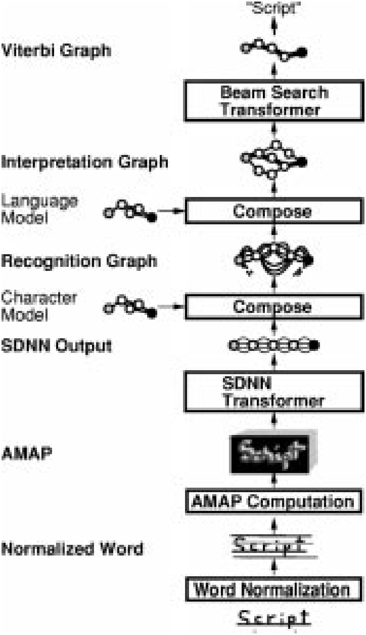
B. Network Architecture
One of the best networks we found for both online and offline character recognition is a five-layer convolutional network somewhat similar to LeNet-5 (Fig. 2), but with multiple input planes and different numbers of units on the last two layers—layer one: convolution with eight kernels of size ; layer two: subsampling; layer three: convolution with 25 kernels of size ; layer four: convolution with 84 kernels of size ; layer five: subsampling; classification layer: 95 RBF units (one per class in the full printable ASCII set). The distributed codes on the output are the same as for LeNet-5, except they are adaptive unlike with LeNet-5. When used in the HOS system, the input to above network consisted of an AMAP with five planes, 20 rows, and 18 columns. It was determined that this resolution was sufficient for representing handwritten characters. In the SDNN version, the number of columns was varied according to the width of the input word. Once the number of subsampling layers and the sizes of the kernels are chosen, the sizes of all the layers, including the input, are determined unambiguously. The only architectural parameters that remain to be selected are the number of feature maps in each layer and the information as to what feature map is connected to what other feature map. In our case, the subsampling rates were chosen as small as possible () and the kernels as small as possible in the first layer () to limit the total number of connections. Kernel sizes in the upper layers are chosen to be as small as possible while satisfying the size constraints mentioned above. Larger architectures did not necessarily perform better and required considerably more time to be trained. A very small architecture with half the input field also performed worse because of insufficient input resolution. Note that the input resolution is nonetheless much less than for OCR because the angle and curvature provide more information than would a single grey level at each pixel.
C. Network Training
Training proceeded in two phases. First, we kept the centers of the RBF’s fixed and trained the network weights so as to minimize the output distance of the RBF unit corresponding to the correct class. This is equivalent to minimizing the MSE between the previous layer and the center of the correct-class RBF. This bootstrap phase was performed on isolated characters. In the second phase, all the parameters, network weights, and RBF centers were trained globally to minimize a discriminative criterion at the word level.
With the HOS approach, the GTN was composed of four main GT’s.
- The segmentation transformer performs the HOS and outputs the segmentation graph. An AMAP is then computed for each image attached to the arcs of this graph.
- The character recognition transformer applies the convolutional network character recognizer to each candidate segment and outputs the recognition graph with penalties and classes on each arc.
- The composition transformer composes the recognition graph with a grammar graph representing a language model incorporating lexical constraints.
- The beam search transformer extracts a good interpretation from the interpretation graph. This task could have been achieved with the usual Viterbi Transformer. The beam search algorithm, however, implements pruning strategies which are appropriate for large interpretation graphs.
With the SDNN approach, the main GT’s are the following.
- The SDNN transformer replicates the convolutional network over the a whole word image and outputs a recognition graph that is a linear graph with class penalties for every window centered at regular intervals on the input image.
- The character-level composition transformer composes the recognition graph with a left-to-right HMM for each character class (as in Fig. 27).
- The word-level composition transformer composes the output of the previous transformer with a language model incorporating lexical constraints and outputs the interpretation graph.
- The beam search transformer extracts a good interpretation from the interpretation graph.
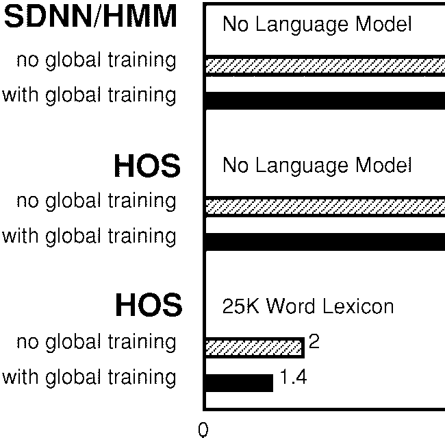
In this application, the language model simply constrains the final output graph to represent sequences of character labels from a given dictionary. Furthermore, the interpretation graph is not actually completely instantiated: the only nodes created are those that are needed by the beam search module. The interpretation graph is therefore represented procedurally rather than explicitly.
A crucial contribution of this research was the joint training of all GT modules within the network with respect to a single criterion, as explained in Sections VI and VII. We used the discriminative forward loss function on the final output graph: minimize the forward penalty of the constrained interpretation (i.e., along all the “correct” paths) while maximizing the forward penalty of the whole interpretation graph (i.e., along all the paths).
During global training, the loss function was optimized with the stochastic diagonal Levenberg–Marquardt procedure described in Appendix C, which uses second derivatives to compute optimal learning rates. This optimization operates on all the parameters in the system, most notably the network weights and the RBF centers.
D. Experimental Results
In the first set of experiments, we evaluated the generalization ability of the NN classifier coupled with the word normalization preprocessing and AMAP input representation. All results are in writer independent mode (different writers in training and testing). Initial training on isolated characters was performed on a database of approximately 100 000 hand printed characters (95 classes of upper case, lower case, digits, and punctuation). Tests on a database of isolated characters were performed separately on the four types of characters: upper case (2.99% error on 9122 patterns), lower case (4.15% error on 8201 patterns), digits (1.4% error on 2938 patterns), and punctuation (4.3% error on 881 patterns). Experiments were performed with the network architecture described above. To enhance the robustness of the recognizer to variations in position, size, orientation, and other distortions, additional training data was generated by applying local affine transformations to the original characters.
The second and third set of experiments concerned the recognition of lower case words (writer independent). The tests were performed on a database of 881 words. First we evaluated the improvements brought by the word normalization to the system. For the SDNN/HMM system we have to use word-level normalization since the network sees one whole word at a time. With the HOS system, and before doing any word-level training, we obtained with character-level normalization 7.3% and 3.5% word and character errors (adding insertions, deletions and substitutions) when the search was constrained within a 25 461-word dictionary. When using the word normalization preprocessing instead of a character level normalization, error rates dropped to 4.6% and 2.0% for word and character errors respectively, i.e., a relative drop of 37% and 43% in word and character error respectively. This suggests that normalizing the word in its entirety is better than first segmenting it and then normalizing and processing each of the segments.
In the third set of experiments, we measured the improvements obtained with the joint training of the NN and the postprocessor with the word-level criterion, in comparison to training based only on the errors performed at the character level. After initial training on individual characters as above, global word-level discriminative training was performed with a database of 3500 lower case words. For the SDNN/HMM system, without any dictionary constraints, the error rates dropped from 38% and 12.4% word and character error to 26% and 8.2% respectively after word-level training, i.e., a relative drop of 32% and 34%.
For the HOS system and a slightly improved architecture, without any dictionary constraints, the error rates dropped from 22.5% and 8.5% word and character error to 17% and 6.3% respectively, i.e., a relative drop of 24.4% and 25.6%. With a 25 461-word dictionary, errors dropped from 4.6% and 2.0% word and character errors to 3.2% and 1.4%, respectively, after word-level training, i.e., a relative drop of 30.4% and 30.0%. Even lower error rates can be obtained by drastically reducing the size of the dictionary to 350 words, yielding 1.6% and 0.94% word and character errors.
These results clearly demonstrate the usefulness of globally trained NN/HMM hybrids for handwriting recognition. This confirms similar results obtained earlier in speech recognition [77].
X A CHECK READING SYSTEM
This section describes a GTN based check reading system, intended for immediate industrial deployment. It also shows how the use of gradient based-learning and GTN’s make this deployment fast and cost-effective while yielding an accurate and reliable solution.
The verification of the amount on a check is a task that is extremely time and money consuming for banks. As a consequence, there is a very high interest in automating the process as much as possible (see, for example, [112]–[114]). Even a partial automation would result in considerable cost reductions. The threshold of economic viability for automatic check readers, as set by the bank, is when 50% of the checks are read with less than 1% error. The other 50% of the check being rejected and sent to human operators. In such a case, we describe the performance of the system as 50% correct/49% reject/1% error. The system presented here was one of the first to cross that threshold on representative mixtures of business and personal checks.
Checks contain at least two versions of the amount. The courtesy amount is written with numerals, while the legal amount is written with letters. On business checks, which are generally machine-printed, these amounts are relatively easy to read but quite difficult to find due to the lack of standard for business check layout. On the other hand, these amounts on personal checks are easy to find but much harder to read.
For simplicity (and speed requirements), our initial task is to read the courtesy amount only. This task consists of two main steps.
- The system has to find, among all the fields (lines of text), the candidates that are the most likely to contain the courtesy amount. This is obvious for many personal checks, where the position of the amount is standardized. However, as already noted, finding the amount can be rather difficult in business checks, even for the human eye. There are many strings of digits, such as the check number, the date, or even “not to exceed” amounts, that can be confused with the actual amount. In many cases, it is very difficult to decide which candidate is the courtesy amount before performing a full recognition.
Figure.
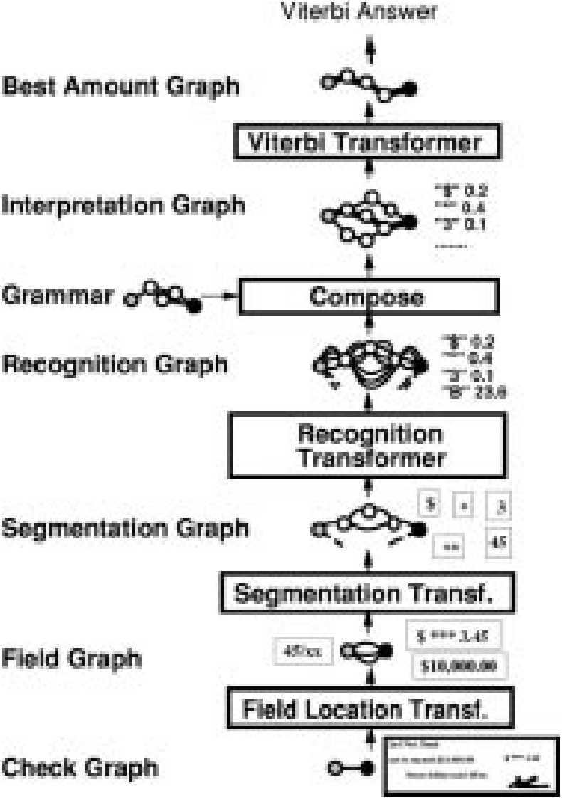
- In order to read (and choose) some courtesy amount candidates, the system has to segment the fields into characters, read and score the candidate characters, and finally find the best interpretation of the amount using contextual knowledge represented by a stochastic grammar for check amounts.
The GTN methodology was used to build a check amount reading system that handles both personal checks and business checks.
A. A GTN for Check Amount Recognition
We now describe the successive graph transformations that allow this network to read the check amount (cf. Fig. 33). Each GT produces a graph whose paths encode and score the current hypotheses considered at this stage of the system.
The input to the system is a trivial graph with a single arc that carries the image of the whole check (cf. Fig. 33).
- The Field Location Transformer: first performs classical image analysis (including connected component analysis, ink density histograms, layout analysis, etc.) and heuristically extracts rectangular zones that may contain the check amount. produces an output graph, called the field graph (cf. Fig. 33) such that each candidate zone is associated with one arc that links the start node to the end node. Each arc contains the image of the zone and a penalty term computed from simple features extracted from the zone (absolute position, size, aspect ratio, etc.). The penalty term is close to zero if the features suggest that the field is a likely candidate and is large if the field is deemed less likely to be an amount. The penalty function is differentiable, therefore its parameters are globally tunable.
An arc may represent separate dollar and cent amounts as a sequence of fields. In fact, in handwritten checks, the cent amount may be written over a fractional bar and not aligned at all with the dollar amount. In the worst case, one may find several cent amount candidates (above and below the fraction bar) for the same dollar amount.
- The Segmentation Transformer: , similar to the one described in Section VIII, examines each zone contained in the field graph and cuts each image into pieces of ink using heuristic image processing techniques. Each piece of ink may be a whole character or a piece of character. Each arc in the field graph is replaced by its corresponding segmentation graph that represents all possible groupings of pieces of ink. Each field segmentation graph is appended to an arc that contains the penalty of the field in the field graph. Each arc carries the segment image, together with a penalty that provides a first evaluation of the likelihood that the segment actually contains a character. This penalty is obtained with a differentiable function that combines a few simple features such as the space between the pieces of ink or the compliance of the segment image with a global baseline, and a few tunable parameters. The segmentation graph represents all the possible segmentations of all the field images. We can compute the penalty for one segmented field by adding the arc penalties along the corresponding path. As before, using a differentiable function for computing the penalties will ensure that the parameters can be optimized globally.
The segmenter uses a variety of heuristics to find candidate cut. One of the most important ones is called “hit and deflect” [115]. The idea is to cast lines downward from the top of the field image. When a line hits a black pixel, it is deflected so as to follow the contour of the object. When a line hits a local minimum of the upper profile, i.e., when it cannot continue downward without crossing a black pixel, it is just propagated vertically downward through the ink. When two such lines meet each other, they are merged into a single cut. The procedure can be repeated from the bottom up. This strategy allows the separation of touching characters such as double zeros.
- The Recognition Transformer: iterates over all segment arcs in the segmentation graph and runs a character recognizer on the corresponding segment image. In our case, the recognizer is LeNet-5, the convolutional NN described in Section II, whose weights constitute the largest and most important subset of tunable parameters. The recognizer classifies segment images into one of 95 classes (fully printable ASCII set) plus a rubbish class for unknown symbols or badly formed characters. Each arc in the input graph is replaced by 96 arcs in the output graph. Each of those 96 arcs contains the label of one of the classes, and a penalty that is the sum of the penalty of the corresponding arc in the input (segmentation) graph, and the penalty associated with classifying the image in the corresponding class, as computed by the recognizer. In other words, the recognition graph represents a weighted trellis of scored character classes. Each path in this graph represents a possible character string for the corresponding field. We can compute a penalty for this interpretation by adding the penalties along the path. This sequence of characters may or may not be a valid check amount.
- The Composition Transformer: selects the paths of the recognition graph that represent valid character sequences for check amounts. This transformer takes two graphs as input: the recognition graph and the grammar graph. The grammar graph contains all possible sequences of symbols that constitute a well-formed amount. The output of the composition transformer, called the interpretation graph, contains all the paths in the recognition graph that are compatible with the grammar. The operation that combines the two input graphs to produce the output is a generalized transduction (see Section IX). A differentiable function is used to compute the data attached to the output arc from the data attached to the input arcs. In our case, the output arc receives the class label of the two arcs and a penalty computed by simply summing the penalties of the two input arcs (the recognizer penalty and the arc penalty in the grammar graph). Each path in the interpretation graph represents one interpretation of one segmentation of one field on the check. The sum of the penalties along the path represents the “badness” of the corresponding interpretation and combines evidence from each of the modules along the process, as well as from the grammar.
- The Viterbi Transformer: The Viterbi transformer finally selects the path with the lowest accumulated penalty corresponding to the best grammatically correct interpretations.
B. Gradient-Based Learning
Each stage of this check reading system contains tunable parameters. While some of these parameters could be manually adjusted (e.g., the parameters of the field locator and segmenter), the vast majority of them must be learned, particularly the weights of the NN recognizer.
Prior to globally optimizing the system, each module parameters are initialized with reasonable values. The parameters of the field locator and the segmenter are initialized by hand, while the parameters of the NN character recognizer are initialized by training on a database of presegmented and labeled characters. Then, the entire system is trained globally from whole check images labeled with the correct amount. No explicit segmentation of the amounts is needed to train the system: it is trained at the check level.
The loss function minimized by our global training procedure is the discriminative forward criterion described in Section VI: the difference between 1) the forward penalty of the constrained interpretation graph (constrained by the correct label sequence) and 2) the forward penalty of the unconstrained interpretation graph. Derivatives can be back propagated through the entire structure, although it is only practical to do it down to the segmenter.
C. Rejecting Low Confidence Checks
In order to be able to reject checks which are the most likely to carry erroneous Viterbi answers, we must rate them with a confidence and reject the check if this confidence is below a given threshold. To compare the unnormalized Viterbi penalties of two different checks would be meaningless when it comes to decide which answer we trust the most.
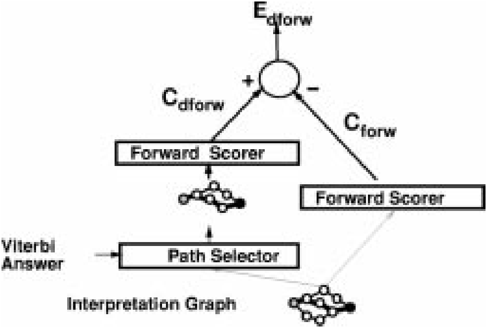
The optimal measure of confidence is the probability of the Viterbi answer given the input image. As seen in Section VI-E, given a target sequence (which, in this case, would be the Viterbi answer), the discriminative forward loss function is an estimate of the logarithm of this probability. Therefore, a simple solution to obtain a good estimate of the confidence is to reuse the interpretation graph (see Fig. 33) to compute the discriminative forward loss as described in Fig. 21, using as our desired sequence the Viterbi answer. This is summarized in Fig. 34, with
D. Results
A version of the above system was fully implemented and tested on machine-print business checks. This system is basically a generic GTN engine with task specific heuristics encapsulated in the check and fprop method. As a consequence, the amount of code to write was minimal: mostly the adaptation of an earlier segmenter into the segmentation transformer. The system that deals with handwritten or personal checks was based on earlier implementations that used the GTN concept in a restricted way.
The NN classifier was initially trained on 500 000 images of character images from various origins spanning the entire printable ASCII set. This contained both handwritten and machine-printed characters that had been previously size normalized at the string level. Additional images were generated by randomly distorting the original images using simple affine transformations of the images. The network was then further trained on character images that had been automatically segmented from check images and manually truthed. The network was also initially trained to reject noncharacters that resulted from segmentation errors. The recognizer was then inserted in the check-reading system and a small subset of the parameters were trained globally (at the field level) on whole check images.
On 646 business checks that were automatically categorized as machine printed, the performance was 82% correctly recognized checks, 1% errors, and 17% rejects. This can be compared to the performance of the previous system on the same test set: 68% correct, 1% errors, and 31% rejects. A check is categorized as machine-printed when characters that are near a standard position dollar sign are detected as machine printed, or when, if nothing is found in the standard position, at least one courtesy amount candidate is found somewhere else. The improvement is attributed to three main causes. First the NN recognizer was bigger and trained on more data. Second, because of the GTN architecture, the new system could take advantage of grammatical constraints in a much more efficient way than the previous system. Third, the GTN architecture provided extreme flexibility for testing heuristics, adjusting parameters, and tuning the system. This last point is more important than it seems. The GTN framework separates the “algorithmic” part of the system from the “knowledge-based” part of the system, allowing easy adjustments of the latter. The importance of global training was only minor in this task because the global training only concerned a small subset of the parameters.
An independent test performed by systems integrators in 1995 showed the superiority of this system over other commercial courtesy amount reading systems. The system was integrated in NCR’s line of check reading systems. It has been fielded in several banks across the United States since June 1996, and it has been reading millions of checks per day since then.
XI CONCLUSIONS
During the short history of automatic pattern recognition, increasing the role of learning seems to have invariably improved the overall performance of recognition systems. The systems described in this paper are more evidence to this fact. Convolutional NN’s have been shown to eliminate the need for hand-crafted feature extractors. GTN’s have been shown to reduce the need for hand-crafted heuristics, manual labeling, and manual parameter tuning in document recognition systems. As training data becomes plentiful, as computers get faster, and as our understanding of learning algorithms improves, recognition systems will rely more and more of learning and their performance will improve.
Just as the back-propagation algorithm elegantly solved the credit assignment problem in multilayer NN’s, the gradient-based learning procedure for GTN’s introduced in this paper solves the credit assignment problem in systems whose functional architecture dynamically changes with each new input. The learning algorithms presented here are in a sense nothing more than unusual forms of gradient descent in complex, dynamic architectures, with efficient back-propagation algorithms to compute the gradient. The results in this paper help establish the usefulness and relevance of gradient-based minimization methods as a general organizing principle for learning in large systems.
It was shown that all the steps of a document analysis system can be formulated as GT’s through which gradients can be back propagated. Even in the nontrainable parts of the system, the design philosophy in terms of graph transformation provides a clear separation between domain-specific heuristics (e.g., segmentation heuristics) and generic, procedural knowledge (the generalized transduction algorithm)
It is worth pointing out that data generating models (such as HMM’s) and the maximum likelihood principle were not called upon to justify most of the architectures and the training criteria described in this paper. Gradient-based learning applied to global discriminative loss functions guarantees optimal classification and rejection without the use of “hard to justify” principles that put strong constraints on the system architecture, often at the expense of performances.
More specifically, the methods and architectures presented in this paper offer generic solutions to a large number of problems encountered in pattern recognition systems.
- Feature extraction is traditionally a fixed transform, and it is generally derived from some expert prior knowledge about the task. This relies on the probably incorrect assumption that the human designer is able to capture all the relevant information in the input. We have shown that the application of gradient-based learning to convolutional NN’s allows us to learn appropriate features from examples. The success of this approach was demonstrated in extensive comparative digit recognition experiments on the NIST database.
- Segmentation and recognition of objects in images cannot be completely decoupled. Instead of taking hard segmentation decisions too early, we have used HOS to generate and evaluate a large number of hypotheses in parallel, postponing any decision until the overall criterion is minimized.
- Hand-truthing images to obtain segmented characters for training a character recognizer is expensive and does not take into account the way in which a whole document or sequence of characters will be recognized (in particular, the fact that some segmentation candidates may be wrong, even though they may look like true characters). Instead we train multinode systems to optimize a global measure of performance, which does not require time consuming detailed hand-truthing and yields significantly better recognition performance because it allows to train these modules to cooperate toward a common goal.
- Ambiguities inherent in the segmentation, character recognition, and linguistic model should be integrated optimally. Instead of using a sequence of task-dependent heuristics to combine these sources of information, we have proposed a unified framework in which generalized transduction methods are applied to graphs representing a weighted set of hypotheses about the input. The success of this approach was demonstrated with a commercially deployed check-reading system that reads millions of business and personal checks per day: the generalized transduction engine resides in only a few hundred lines of code.
- Traditional recognition systems rely on many hand-crafted heuristics to isolate individually recognizable objects. The promising SDNN approach draws on the robustness and efficiency of convolutional NN’s to avoid explicit segmentation altogether. Simultaneous automatic learning of segmentation and recognition can be achieved with gradient-based learning methods.
This paper presents a small number of examples of GT modules, but it is clear that the concept can be applied to many situations where the domain knowledge or the state information can be represented by graphs. This is the case in many audio signal recognition tasks, and visual scene analysis applications. Future work will attempt to apply GT networks to such problems, with the hope of allowing more reliance on automatic learning and less on detailed engineering.
Appendix a Preconditions for Faster Convergence
As seen before, the squashing function used in our convolutional networks is . Symmetric functions are believed to yield faster convergence, although the learning can become extremely slow if the weights are too small. The cause of this problem is that in weight space the origin is a fixed point of the learning dynamics and, although it is a saddle point, it is attractive in almost all directions [116]. For our simulations, we use and (see [20], [34]). With this choice of parameters, the equalities and are satisfied. The rationale behind this is that the overall gain of the squashing transformation is around one in normal operating conditions, and the interpretation of the state of the network is simplified. Moreover, the absolute value of the second derivative of is a maximum at and , which improves the convergence toward the end of the learning session. This particular choice of parameters is merely a convenience, and does not affect the result.
Before training, the weights are initialized with random values using a uniform distribution between and , where is the number of inputs (fan-in) of the unit which the connection belongs to. Since several connections share a weight, this rule could be difficult to apply, but in our case all connections sharing a same weight belong to units with identical fan-ins. The reason for dividing by the fan-in is that we would like the initial standard deviation of the weighted sums to be in the same range for each unit and to fall within the normal operating region of the sigmoid. If the initial weights are too small, the gradients are very small and the learning is slow. If they are too large, the sigmoids are saturated and the gradient is also very small. The standard deviation of the weighted sum scales like the square root of the number of inputs when the inputs are independent, and it scales linearly with the number of inputs if the inputs are highly correlated. We chose to assume the second hypothesis since some units receive highly correlated signals.
Appendix B Stochastic Gradient Versus Batch Gradient
Gradient-based learning algorithms can use one of two classes of methods to update the parameters. The first method, dubbed “batch gradient,” is the classical one: the gradients are accumulated over the entire training set, and the parameters are updated after the exact gradient has been so computed. In the second method, called “stochastic gradient,” a partial, or noisy, gradient is evaluated on the basis of one single training sample (or a small number of samples), and the parameters are updated using this approximate gradient. The training samples can be selected randomly or according to a properly randomized sequence. In the stochastic version the gradient estimates are noisy, but the parameters are updated much more often than with the batch version. An empirical result of considerable practical importance is that on tasks with large, redundant data sets, the stochastic version is considerably faster than the batch version, sometimes by orders of magnitude [117]. Although the reasons for this are not totally understood theoretically, an intuitive explanation can be found in the following extreme example. Let us take an example where the training database is composed of two copies of the same subset. Then accumulating the gradient over the whole set would cause redundant computations to be performed. On the other hand, running Stochastic Gradient once on this training set would amount to performing two complete learning iterations over the small subset. This idea can be generalized to training sets where there exist no precise repetition of the same pattern but where some redundancy is present. In fact stochastic update must be better when there is redundancy, i.e., when a certain level of generalization is expected.
Many authors have claimed that second-order methods should be used in lieu of gradient descent for NN training. The literature abounds with recommendations [118] for classical second-order methods such as the Gauss–Newton or Levenberg–Marquardt algorithms for quasi-Newton methods such as Broyden–Fletcher–Goldfarb–Shanno, limited-storage Broyden–Fletcher–Goldfarb–Shanno, or for various versions of the conjugate gradients method. Unfortunately, all of the above methods are unsuitable for training large NN’s on large data sets. The Gauss–Newton and Levenberg–Marquardt methods require operations per update, where is the number of parameters, which makes them impractical for even moderate size networks. Quasi-Newton methods require “only” operations per update, but that still makes them impractical for large networks. Limited-storage Broyden–Fletcher–Goldfarb–Shanno’s and conjugate gradients require only operations per update so they would appear appropriate. Unfortunately, their convergence speed relies on an accurate evaluation of successive “conjugate descent directions” which only makes sense in “batch” mode. For large data sets, the speed-up brought by these methods over regular batch gradient descent cannot match the enormous speed up brought by the use of stochastic gradient. Several authors have attempted to use conjugate gradient with small batches or batches of increasing sizes [119], [120], but those attempts have not yet been demonstrated to surpass a carefully tuned stochastic gradient. Our experiments were performed with a stochastic method that scales the parameter axes so as to minimize the eccentricity of the error surface.
Appendix C Stochastic Diagonal Levenberg–marquardt
Owing to the reasons given in Appendix B, we prefer to update the weights after each presentation of a single pattern in accordance with stochastic update methods. The patterns are presented in a constant random order, and the training set is typically repeated 20 times.
Our update algorithm is dubbed the stochastic diagonal Levenberg–Marquardt method where an individual learning rate (step size) is computed for each parameter (weight) before each pass through the training set [20], [34], [121]. These learning rates are computed using the diagonal terms of an estimate of the Gauss–Newton approximation to the Hessian (second derivative) matrix. This algorithm is not believed to bring a tremendous increase in learning speed but it converges reliably without requiring extensive adjustments of the learning parameters. It corrects major ill-conditioning of the loss function that are due to the peculiarities of the network architecture and the training data. The additional cost of using this procedure over standard stochastic gradient descent is negligible.
At each learning iteration a particular parameter is updated according to the following stochastic update rule:
where is the instantaneous loss function for pattern . In convolutional NN’s, because of the weight sharing, the partial derivative is the sum of the partial derivatives with respect to the connections that share the parameter
where is the connection weight from unit to unit , is the set of unit index pairs such that the connection between and share the parameter , i.e.,
As stated previously, the step sizes are not constant but are function of the second derivative of the loss function along the axis
where is a hand-picked constant and is an estimate of the second derivative of the loss function with respect to . The larger is, the smaller the weight update. The parameter prevents the step size from becoming too large when the second derivative is small, very much like the “model-trust” methods, and the Levenberg–Marquardt methods in nonlinear optimization [8]. The exact formula to compute from the second derivatives with respect to the connection weights is
However, we make three approximations. The first approximation is to drop the off-diagonal terms of the Hessian with respect to the connection weights in (22)
Naturally, the terms are the average over the training set of the local second derivatives
Those local second derivatives with respect to connection weights can be computed from local second derivatives with respect to the total input of the downstream unit
where is the state of unit and is the second derivative of the instantaneous loss function with respect to the total input to unit (denoted ). Interestingly, there is an efficient algorithm to compute those second derivatives which is very similar to the back-propagation procedure used to compute the first derivatives [20], [21]
Unfortunately, using those derivatives leads to well-known problems associated with every Newton-like algorithm: these terms can be negative and can cause the gradient algorithm to move uphill instead of downhill. Therefore, our second approximation is a well-known trick called the Gauss–Newton approximation, which guarantees that the second derivative estimates are nonnegative. The Gauss–Newton approximation essentially ignores the nonlinearity of the estimated function (the NN, in our case), but not that of the loss function. The back propagation equation for Gauss-Newton approximations of the second derivatives is
This is very similar to the formula for back propagating the first derivatives, except that the sigmoid’s derivative and the weight values are squared. The right-hand side is a sum of products of nonnegative terms, therefore the left-hand side term is nonnegative.
The third approximation we make is that we do not run the average in (24) over the entire training set, but run it on a small subset of the training set instead. In addition the re-estimation does not need to be done often since the second-order properties of the error surface change rather slowly. In the experiments described in this paper, we re-estimate the on 500 patterns before each training pass through the training set. Since the size of the training set is 60 000, the additional cost of re-estimating the is negligible. The estimates are not particularly sensitive to the particular subset of the training set used in the averaging. This seems to suggest that the second-order properties of the error surface are mainly determined by the structure of the network, rather than by the detailed statistics of the samples. This algorithm is particularly useful for shared-weight networks because the weight sharing creates ill conditioning of the error surface. Because of the sharing, one single parameter in the first few layers can have an enormous influence on the output. Consequently, the second derivative of the error with respect to this parameter may be very large, while it can be quite small for other parameters elsewhere in the network. The above algorithm compensates for that phenomenon.
Unlike most other second-order acceleration methods for back-propagation, the above method works in stochastic mode. It uses a diagonal approximation of the Hessian. Like the classical Levenberg–Marquardt algorithm, it uses a “safety” factor to prevent the step sizes from getting too large if the second derivative estimates are small. Hence the method is called the stochastic diagonal Levenberg–Marquardt method.
Acknowledgments
Some of the systems described in this paper are the work of many researchers now at AT&T and Lucent Technologies. In particular, C. Burges, C. Nohl, T. Cauble, and J. Bromley contributed much to the check reading system. Experimental results described in Section III include contributions by C. Burges, A. Brunot, C. Cortes, H. Drucker, L. Jackel, U. Müller, B. Schölkopf, and P. Simard. The authors wish to thank F. Pereira, V. Vapnik, J. Denker, and I. Guyon for helpful discussions, C. Stenard and R. Higgins for providing the applications that motivated some of this work, and L. R. Rabiner and L. D. Jackel for relentless support and encouragement.