Depth-First Search and Linear Graph Algorithms

Robert Tarjan†

Abstract. The value of depth-first search or “backtracking” as a technique for solving problems is illustrated by two examples. An improved version of an algorithm for finding the strongly connected components of a directed graph and an algorithm for finding the biconnected components of an undirect graph are presented. The space and time requirements of both algorithms are bounded by $k_1 V + k_2 E + k_3$ for some constants $k_1, k_2,$ and $k_3$, where $V$ is the number of vertices and $E$ is the number of edges of the graph being examined.

Key words. Algorithm, backtracking, biconnectivity, connectivity, depth-first, graph, search, spanning tree, strong-connectivity.

1. Introduction. Consider a graph $G$, consisting of a set of vertices $\mathcal{V}$ and a set of edges $\mathcal{E}$. The graph may either be directed (the edges are ordered pairs $(v, w)$ of vertices; $v$ is the tail and $w$ is the head of the edge) or undirected (the edges are unordered pairs of vertices, also represented as $(v, w)$). Graphs form a suitable abstraction for problems in many areas; chemistry, electrical engineering, and sociology, for example. Thus it is important to have the most economical algorithms for answering graph-theoretical questions.

In studying graph algorithms we cannot avoid at least a few definitions. These definitions are more-or-less standard in the literature. (See Harary [3], for instance.) If $G = (\mathcal{V}, \mathcal{E})$ is a graph, a path $p : v \Rightarrow^* w$ in $G$ is a sequence of vertices and edges leading from $v$ to $w$. A path is simple if all its vertices are distinct. A path $p : v \Rightarrow^* v$ is called a closed path. A closed path $p : v \Rightarrow^* v$ is a cycle if all its edges are distinct and the only vertex to occur twice in $p$ is $v$, which occurs exactly twice. Two cycles which are cyclic permutations of each other are considered to be the same cycle. The undirected version of a directed graph is the graph formed by converting each edge of the directed graph into an undirected edge and removing duplicate edges. An undirected graph is connected if there is a path between every pair of vertices.

A (directed rooted) tree $T$ is a directed graph whose undirected version is connected, having one vertex which is the head of no edges (called the root), and such that all vertices except the root are the head of exactly one edge. The relation “$(v, w)$ is an edge of $T$” is denoted by $v \rightarrow w$. The relation “There is a path from $v$ to $w$ in $T$” is denoted by $v \Rightarrow^* w$. If $v \rightarrow w$, $v$ is the father of $w$ and $w$ is a son of $v$. If $v \Rightarrow^* w$, $v$ is an ancestor of $w$ and $w$ is a descendant of $v$. Every vertex is an ancestor and a descendant of itself. If $v$ is a vertex in a tree $T$, $T_v$ is the subtree of $T$ having as vertices all the descendants of $v$ in $T$. If $G$ is a directed graph, a tree $T$ is a spanning tree of $G$ if $T$ is a subgraph of $G$ and $T$ contains all the vertices of $G$.

If $R$ and $S$ are binary relations, $R^*$ is the transitive closure of $R$, $R^{-1}$ is the inverse of $R$, and

* Received by the editors August 30, 1971, and in revised form March 9, 1972. † Department of Computer Science, Cornell University, Ithaca, New York 14850. This research was supported by the Hertz Foundation and the National Science Foundation under Grant GJ-992.

If $f, f_1, \cdots, f_n$ are functions of $x_1, \cdots, x_n$, we say $f$ is $O(f_1, \cdots, f_n)$ if

for all $x_i$ and some constants $k_0, \cdots, k_n$. We shall assume a random-access computer model.

1. Depth-first search. Backtracking, or depth-first search, is a technique which has been widely used for finding solutions to problems in combinatorial theory and artificial intelligence [2], [11] but whose properties have not been widely analyzed. Suppose $G$ is a graph which we wish to explore. Initially all the vertices of $G$ are unexplored. We start from some vertex of $G$ and choose an edge to follow. Traversing the edge leads to a new vertex. We continue in this way; at each step we select an unexplored edge leading from a vertex already reached and we traverse this edge. The edge leads to some vertex, either new or already reached. Whenever we run out of edges leading from old vertices, we choose some unreached vertex, if any exists, and begin a new exploration from this point. Eventually we will traverse all the edges of $G$, each exactly once. Such a process is called a search of $G$.

There are many ways of searching a graph, depending upon the way in which edges to search are selected. Consider the following choice rule: when selecting an edge to traverse, always choose an edge emanating from the vertex most recently reached which still has unexplored edges. A search which uses this rule is called a depth-first search. The set of old vertices with possibly unexplored edges may be stored on a stack. Thus a depth-first search is very easy to program either iteratively or recursively, provided we have a suitable computer representation of a graph.

Definition 1. Let $G = (\mathcal{V}, \mathcal{E})$ be a graph. For each vertex $v \in \mathcal{V}$ we may construct a list containing all vertices $w$ such that $(v, w) \in \mathcal{E}$. Such a list is called an adjacency list for vertex $v$. A set of such lists, one for each vertex in $G$, is called an adjacency structure for $G$.

If the graph $G$ is undirected, each edge $(v, w)$ is represented twice in an adjacency structure; once for $v$ and once for $w$. If $G$ is directed, each edge $(v, w)$ is represented once: vertex $w$ appears in the adjacency list of vertex $v$. A single graph may have many adjacency structures; in fact, each ordering of the edges around the vertices of $G$ gives a unique adjacency structure, and each adjacency structure corresponds to a unique ordering of the edges at each vertex. Using an adjacency structure for a graph, we can perform depth-first searches in a very efficient manner, as we shall see.

Suppose $G$ is a connected undirected graph. A search of $G$ imposes a direction on each edge of $G$ given by the direction in which the edge is traversed when the search is performed. Thus $G$ is converted into a directed graph $G'$. The set of edges which lead to a new vertex when traversed during the search defines a spanning tree of $G'$. In general, the arcs of $G'$ which are not part of the spanning tree interconnect the paths in the tree. However, if the search is depth-first, each edge $(v, w)$ not in the spanning tree connects vertex $v$ with one of its ancestors $w$.

Definition 2. Let $P$ be a directed graph, consisting of two disjoint sets of edges, denoted by $v \to w$ and $v \longrightarrow w$ respectively. Suppose $P$ satisfies the following properties: {#tarjan-1972-dfs-def-2 .statement tag=03E4} (i) The subgraph $T$ containing the edges $v \to w$ is a spanning tree of $P$.

(ii) We have $-\rightarrow \subseteq (\rightarrow^*)^{-1}$, where “$\rightarrow$” and “$-\rightarrow$” denote the relations defined by the corresponding set of edges. That is, each edge which is not in the spanning tree $T$ of $P$ connects a vertex with one of its ancestors in $T$. Then $P$ is called a palm tree. The edges $v \rightarrow w$ are called the fronds of $P$.

Theorem 1. Let $P$ be the directed graph generated by a depth-first search of a connected graph $G$. Then $P$ is a palm tree. Conversely, let $P$ be any palm tree. Then $P$ is generated by some depth-first search of the undirected version of $P$.

Proof. Consider the program listed below, which carries out a depth-first search of a connected graph, starting at vertex $s$, using an adjacency structure of the graph to be searched. The program numbers the vertices of the graph in the order they are reached during the search and constructs the directed graph $(P)$ generated by the search.

            
              BEGIN
INTEGER i;
PROCEDURE DFS(v, u); COMMENT vertex u is the father of vertex v in the spanning tree being constructed;
BEGIN
NUMBER (v) := i := i + 1;
FOR w in the adjacency list of v DO
BEGIN
IF w is not yet numbered THEN
BEGIN
construct arc v → w in P;
DFS(w, v);
END
ELSE IF NUMBER (w) < NUMBER (v) and w → = u THEN construct arc v → w in p;
END;
i := 0;
DFS(s, 0);
END;
            
          

Figure 1 gives an example of the application of DFS to a graph. Suppose $P = (\mathcal{V}, \mathcal{E})$ is the directed graph generated by a depth-first search of some connected graph $G$, and assume that the search begins at vertex $s$. Examine the procedure DFS. The algorithm clearly terminates because each vertex can only be numbered once. Furthermore, each edge in the graph is examined exactly twice. Therefore the time required by the search is linear in $V$ and $E$.

For any vertices $v$ and $w$, let $d(v, w)$ be the length of the shortest path between $v$ and $w$ in $G$. Since $G$ is connected, all distances are finite. Suppose that some vertex remains unnumbered by the search. Let $v$ be an unnumbered vertex such that $d(s, v)$ is minimal. Then there is a vertex $w$ such that $w$ is adjacent to $v$ and $d(s, w) < d(s, v)$. Thus $w$ is numbered. But $v$ will also be numbered, since it is adjacent to $w$. This means that all vertices are numbered during the search.

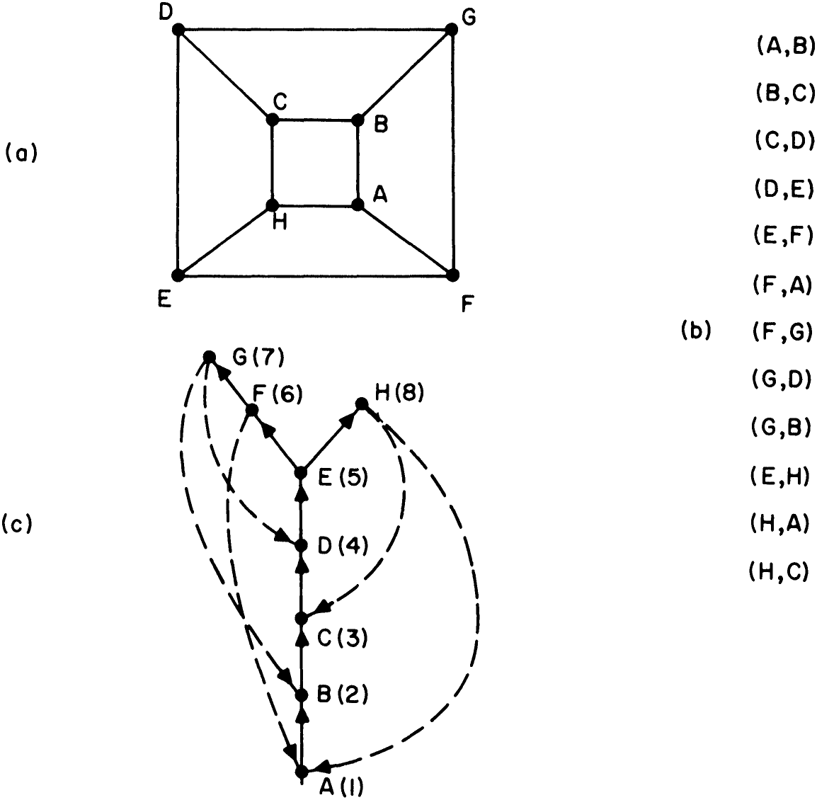
(a) The graph (b) Order of edge exploration (c) Generated palm tree, with numbers of vertices in ( )

The vertex s is the head of no edge w → s. Each other vertex v is the head of exactly one edge w → v. The subgraph T of P defined by the edges v → w is obviously connected. Thus T is a spanning tree of P.

Each arc of the original graph is directed in at least one direction; if (v, w) does not become an arc of the spanning tree T, either v → w or w → v must be constructed since both v and w are numbered whenever edge (v, w) is inspected and either NUMBER (v) < NUMBER (w) or NUMBER (v) > NUMBER (w).

The arcs v → w run from smaller numbered points to larger numbered points. The arcs v → w run from larger numbered points to smaller numbered points. If arc v → w is constructed, arc w → v is not constructed later because v is numbered. If arc w → v is constructed, arc v → w is not later constructed, because of the test “w — = u” in procedure DFS. Thus each edge in the original graph is directed in one and only one direction.

Consider an arc v → w. We have NUMBER (w) < NUMBER (v). Thus w is numbered before v. Since v → w is constructed and not w → v, v must be numbered before edge (w, v) is inspected. Thus v must be numbered during execution of DFS $(w, -)$. But all vertices numbered during execution of DFS $(w, -)$ are descendants of $w$. This means that $w \rightarrow^* v$, and $G$ is a palm tree.

Let us prove the converse part of the theorem. Suppose that $P$ is a palm tree, with spanning tree $T$ and undirected version $G$. Construct an adjacency structure of $G$ in which all the edges of $T$ appear before the other edges of $G$ in the adjacency lists. Starting with the root of $T$, perform a depth-first search using this adjacency structure. The search will traverse the edges of $T$ preferentially and will generate the palm tree $P$; it is easy to see that each edge is directed correctly. This completes the proof of the theorem.

We may state Theorem 1 nonconstructively as the following corollary.

Corollary 2. Let $G$ be any undirected graph. Then $G$ can be converted into a palm tree by directing its edges in a suitable manner.

1. Biconnectivity. The value of depth-first search follows from the simple structure of a palm tree. Let us consider a problem in which this structure is useful.

Definition 3. Let $G = (\mathcal{V}, \mathcal{E})$ be an undirected graph. Suppose that for each triple of distinct vertices $v, w, a$ in $\mathcal{V}$, there is a path $p : v \Rightarrow^* w$ such that $a$ is not on the path $p$. Then $G$ is biconnected. (Other equivalent definitions of biconnectedness exist.) If, on the other hand, there is a triple of distinct vertices $v, w, a$ in $\mathcal{V}$ such that $a$ is on any path $p : v \Rightarrow^* w$, and there exists at least one such path, then $a$ is called an articulation point of $G$.

Lemma 3. Let $G = (\mathcal{V}, \mathcal{E})$ be an undirected graph. We may define an equivalence relation on the set of edges as follows: two edges are equivalent if and only if they belong to a common cycle. Let the distinct equivalence classes under this relation be $\mathcal{E}_i, 1 \leq i \leq n$, and let $G_i = (\mathcal{V}_i, \mathcal{E}_i)$, where $\mathcal{V}_i$ is the set of vertices incident to the edges of $\mathcal{E}_i$; $\mathcal{V}_i = \{v | \exists w ((v, w) \in \mathcal{E}_i)\}$. Then: {#tarjan-1972-dfs-lem-3 .statement tag=03E9} (i) $G_i$ is biconnected, for each $1 \leq i \leq n$. (ii) No $G_i$ is a proper subgraph of a biconnected subgraph of $G$. (iii) Each articulation point of $G$ occurs more than once among the $\mathcal{V}_i, 1 \leq i \leq n$. Each nonarticulation point of $G$ occurs exactly once among the $\mathcal{V}_i, 1 \leq i \leq n$. (iv) The set $\mathcal{V}_i \cap \mathcal{V}_j$ contains at most one point, for any $1 \leq i, j \leq n$. Such a point of intersection is an articulation point of the graph.

The subgraphs $G_i$ of $G$ are called the biconnected components of $G$.

Suppose we wish to determine the biconnected components of an undirected graph $G$. Common algorithms for this purpose, for instance, Shirey's [14], test each vertex in turn to discover if it is an articulation point. Such algorithms require time proportional to $V \cdot E$, where $V$ is the number of vertices and $E$ is the number of edges of the graph. A more efficient algorithm uses depth-first search. Let $P$ be a palm tree generated by a depth-first search. Suppose the vertices of $P$ are numbered in the order they are reached during the search (as is done by the procedure DFS above). We shall refer to vertices by their numbers. If $u$ is an ancestor of $v$ in the spanning tree $T$ of $P$, then $u < v$. For any vertex $v$ in $P$, let LOWPT $(v)$ be the smallest vertex in the set $\{v\} \cup \{w | v \rightarrow^* \rightarrow w\}$. That is, LOWPT $(v)$ is the smallest vertex reachable from $v$ by traversing zero or more tree arcs followed by at most one frond. The following results form the basis of an efficient algorithm for finding biconnected components. This algorithm was discovered by Hopcroft and Tarjan [4]. Paton [12] describes a similar algorithm.

Lemma 4. Let G be an undirected graph and let P be a palm tree formed by directing the edges of G. Let T be the spanning tree of P. Suppose p : v $\Rightarrow *$ w is any path in G. Then p contains a point which is an ancestor of both v and w in T.

Proof. Let $T_u$ with root u be the smallest subtree of T containing all vertices on the path p. If $u = v$ or $u = w$, the lemma is immediate. Otherwise, let $T_{u_1}$ and $T_{u_2}$ be two distinct subtrees containing points on p such that $u \rightarrow u_1$ and $u \rightarrow u_2$. If only one such subtree exists, then u is on p since $T_u$ is minimal. If two such subtrees exist, path p can only get from $T_{u_1}$ to $T_{u_2}$ by passing through vertex u, since no point in one of these trees is an ancestor of any point in the other, while both $\rightarrow$ and $\longrightarrow$ connect only ancestors in a palm tree. Since u is an ancestor of both v and w, the lemma holds.

Lemma 5. Let G be a connected undirected graph. Let P be a palm tree formed by directing the edges of G, and let T be the spanning tree of P. Suppose a, v, w are distinct vertices of G such that $(a, v) \in T$, and suppose w is not a descendant of v in T. (That is, $\neg (v \Rightarrow * w)$ in T.) If $\mathrm{LOWPT}(v) \geq a$, then a is an articulation point of P and removal of a disconnects v and w. Conversely, if a is an articulation point of G, then there exist vertices v and w which satisfy the properties above.

Proof. If $a \rightarrow v$ and $\mathrm{LOWPT}(v) \geq a$, then any path from v not passing through a remains in the subtree $T_v$, and this subtree does not contain the point w. This gives the first part of the lemma.

To prove the converse, let a be an articulation point of G. If a is the root of P, then at least two tree arcs must emanate from a. Let v be the head of one such arc and let w be the head of another such arc. Then $a \rightarrow v$, $\mathrm{LOWPT}(v) \geq a$, and w is not a descendant of v. If a is not the root of P, consider the connected components formed by deleting a from G. One component must consist only of descendants of a. Such a component can contain only one son of v by Lemma 4. Let v be such a son of a. Let w be any proper ancestor of a. Then $a \rightarrow v$, $\mathrm{LOWPT}(v) \geq a$, and w is not a descendant of v. Thus the converse part of the lemma is true.

Corollary 6. Let G be a connected undirected graph, and let P be a palm tree formed by directing the edges of G. Suppose that P has a spanning tree T. If C is a biconnected component of G, then the vertices of C define a subtree of T, and the root of this subtree is either an articulation point of G or is the root of T.

Figure 2 shows a graph, its LOWPT values, articulation points, and biconnected components. The LOWPT values of all the vertices of a palm tree P may be calculated during a single depth-first search, since

On the basis of such a calculation, the articulation points and the biconnected components may be determined, all during one search. The biconnectivity algorithm is presented below. The program will compute the biconnected components

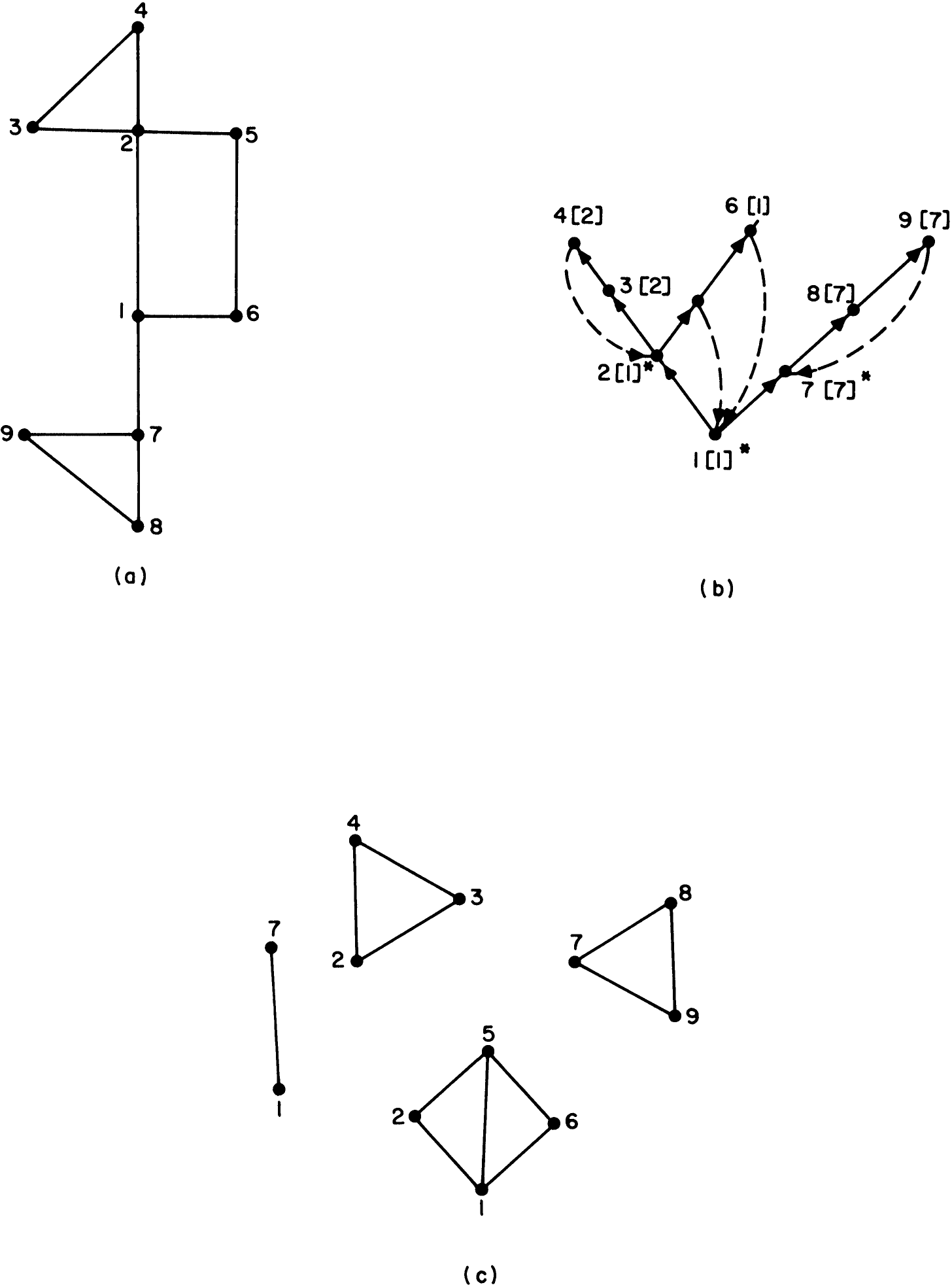
(a) Graph (b) A palm tree with LOWPT values in [ ], articulation points marked with * (c) Biconnected components of a graph $G$, starting from vertex $s$.

            
              BEGIN
    INTEGER i;
    procedure BICONNECT (v, u);
        BEGIN
            NUMBER (v) := i := i + 1;
            LOWPT (v) = NUMBER (v);
            FOR w in the adjacency list of v DO
                BEGIN
                    IF w is not yet numbered THEN
                        BEGIN
                            add (v, w) to stack of edges;
                            BICONNECT (w, v)
                            LOWPT (v) := min (LOWPT (v), LOWPT (w));
                            IF LOWPT (w) ≥ NUMBER (v) THEN
                                BEGIN
                                    start new biconnected component;
                                    WHILE top edge e = (u₁, u₂) on edge stack has NUMBER (u₁) ≥ NUMBER (w) DO
                                        delete (u₁, u₂) from edge stack and add it to current component;
                                        delete (v, w) from edge stack and add it to current component;
                                END;
                        END
                    ELSE IF (NUMBER (w) < NUMBER (v)) and (w → = u) THEN
                        BEGIN
                            add (v, w) to edge stack;
                            LOWPT (v) := min (LOWPT (v), NUMBER (w));
                        END;
                END;
            END;
        END;
    i := 0;
    empty the edge stack;
    FOR w a vertex DO IF w is not yet numbered THEN BICONNECT (w, 0);
END;
            
          

The edges of $G$ are placed on a stack as they are traversed; when an articulation point is found the corresponding edges are all on top of the stack. (If $(v, w) \in T$ and $\mathrm{LOWPT}(w) \geq \mathrm{LOWPT}(v)$, then the corresponding biconnected component contains the edges in $\{(u_1, u_2)|w \rightarrow^* u_1\} \cup \{(v, w)\}$ which are on the edge stack.) A single search on each connected component of a graph $G$ will give us all the connected components of $G$.

THEOREM 7. The biconnectivity algorithm requires $O(V, E)$ space and time when applied to a graph with $V$ vertices and $E$ edges.

Proof. The algorithm clearly requires space bounded by $k_1 V + k_2 E + k_3$, for some constants $k_1, k_2,$ and $k_3$. The algorithm is an elaboration of the depth-first search procedure DFS. During the search, LOWPT values are calculated and each edge is placed on the edge stack once and removed from the edge stack once. The amount of extra time required by these operations is proportional to $E$. Thus BICONNECT has a time bound linear in $V$ and $E$.

Theorem 8. The biconnectivity algorithm correctly gives the biconnected components of any undirected graph G.

Proof. The actual depth-first search undertaken by the algorithm depends on the adjacency structure chosen to represent $G$; we shall prove that the algorithm is correct for all adjacency structures. Notice first that the biconnectivity algorithm analyzes each connected component of $G$ separately to find its biconnected components, applying one depth-first search to each connected component. Thus we need only prove that the biconnectivity algorithm works correctly on connected graphs $G$.

The correctness proof is by induction on the number of edges in $G$. Suppose $G$ is connected and contains no edges. $G$ either is empty or consists of a single point. The algorithm will terminate after examining $G$ and listing no components. Thus the algorithm operates correctly in this case. Now suppose that the algorithm works correctly on all connected graphs with $E - 1$ or fewer edges. Consider applying the algorithm to a connected graph $G$ with $E$ edges.

Each edge placed on the stack of edges is eventually removed and added to a component since everything on the edge stack is removed whenever the search returns to the root of the palm tree of $G$. Consider the situation when the first component $G'$ is formed. Suppose that this component does not include all the edges of $G$. Then the vertex $v$ currently being examined is an articulation point of the graph and separates the edges in the component from the other edges in the graph by Lemma 5.

Consider only the set of edges in the component. If BICONNECT $(v, 0)$ is executed, using the graph $G'$ as data, the steps taken by the algorithm are the same as those taken during the analysis of the edges of $G'$ when the data consists of the entire graph $G$. Since $G'$ contains fewer edges than $G$, the algorithm operates correctly on $G'$ and $G'$ must be biconnected. If we delete the edges of $G'$ from $G$, we get another subgraph $G''$ with fewer edges than $G$ since $G'$ is not empty. The algorithm operates correctly on $G''$ by the induction assumption. The behavior of the algorithm on $G$ is simply a composite of its behavior on $G'$ and on $G''$; thus the algorithm must operate correctly on $G$.

Now suppose that only one component is found. We want to show that in this case $G$ is biconnected. Suppose that $G$ is not biconnected. Then $G$ has an articulation point $a$. By Lemma 5, LOWPT $(v) \geq a$ for some son $v$ of $a$. But the articulation point test in the program will succeed when the edge $(a, v)$ is examined, and more than one biconnected component will be generated. This contradiction shows that $G$ is biconnected, and the algorithm works correctly in this case.

By induction, the biconnectivity algorithm gives the correct components when applied to any connected graph, and hence when applied to any graph.

1. Strong connectivity. The biconnectivity algorithm shows how useful depth-first search can be when applied to undirected graphs. However, when a directed graph is searched in a depth-first manner, a simple palm tree structure does not result, because the direction of search on each edge is fixed. The more complicated structure which results in this case is still simple enough to prove useful in at least one application.

Definition 4. Let G be a directed graph. Suppose that for each pair of vertices v, w in G, there exist paths $p_1 : v \Rightarrow^* w$ and $p_2 : w \Rightarrow^* v$. Then G is said to be strongly connected.

Lemma 9. *Let $G = (\mathcal{V}, \mathcal{E})$ be a directed graph. We may define an equivalence relation on the set of vertices as follows: two vertices v and w are equivalent if there is a closed path $p : v \Rightarrow^* v$ which contains w. Let the distinct equivalence classes under this relation be $\mathcal{V}_i, 1 \leq i \leq n$. Let $G_i = (\mathcal{V}_i, \mathcal{E}_i)$, where $\mathcal{E}_i = \{(v, w) \in \mathcal{E} | v, w \in \mathcal{V}_i\}$. Then:

(i) Each $G_i$ is strongly connected. (ii) No $G_i$ is a proper subgraph of a strongly connected subgraph of G.*

The subgraphs $G_i$ are called the strongly connected components of G.

Suppose we wish to determine the strongly connected components of a directed graph. This problem is related to the problem of determining the ergodic subchains and transient states of a Markov chain. Fox and Landy [1] give an algorithm for solving the latter problem; Purdom [13] and Munro [10] present virtually identical methods for solving the former problem. These algorithms use depth-first search. Purdom claims a time bound of $k V^2$ for his algorithm; Munro claims $k \max (E, V \log V)$, where the graph has $V$ vertices and $E$ edges. Their algorithm attempts to construct a cycle by starting from a point and beginning a depth-first search. When a cycle is found, the vertices on the cycle are marked as being in the same strongly connected component and the process is repeated. The algorithm has the disadvantage that two small strongly connected components may be collapsed into a bigger one; the resultant extra work in relabeling may contribute $V^2$ steps using a simple approach, or $V \log V$ steps if a more sophisticated approach is used (see Munro [10]). In fact, the time bound may be reduced further if an efficient list merging algorithm [9] is used. However, a more careful study of what a depth-first search does to a directed graph reveals that an $O(V, E)$ algorithm which requires no merging of components may be devised.

Consider what happens when a depth-first search is performed on a directed graph $G$. The set of edges which lead to a new vertex when traversed during the search form a tree. The other edges fall into three classes. Some are edges running from ancestors to descendants in the tree. These edges may be ignored, because they do not affect the strongly connected components of $G$. Some edges run from descendants to ancestors in the tree; these we may call fronds as above. Other edges run from one subtree to another in the tree. These, we call cross-links. It is easy to verify that if the vertices of the tree are numbered in the order they are reached during the search, a cross-link $(v, w)$ always has $\mathrm{NUMBER}(v) > \mathrm{NUMBER}(w)$. We shall denote tree edges by $v \rightarrow w$, and fronds and cross-links by $v \rightarrow w$.

Suppose $G$ is a directed graph, to which a depth-first search algorithm is applied repeatedly until all the edges are explored. The process will create a set of trees which contain all the vertices of $G$, called the spanning forest $F$ of $G$, and sets of fronds and cross-links. (Other edges are thrown away.) A directed graph consisting of a spanning forest and sets of fronds and cross-links is called a jungle. Suppose the vertices are numbered in the order they are reached during the search and that we refer to vertices by their number. Then we have the following results.

Lemma 10. Let v and w be vertices in G which lie in the same strongly connected component. Let F be a spanning forest of G generated by repeated depth-first search. Then v and w have a common ancestor in F. Further, if u is the highest numbered common ancestor of v and w, then u lies in the same strongly connected component as v and w.

Proof. Without loss of generality we may assume $v \leq w$. Let p be a path from v to w in G. Let $T_u$ with root u be the smallest subtree of a tree in F containing all the vertices in p. There must be such a tree, since p can pass from one tree in F to another tree with smaller numbered vertices but p can never lead to a tree with larger numbered vertices. If p were contained in two or more trees of F, it could not end at w, since $v \leq w$.

Thus $T_u$ exists, and v and w have a common ancestor in F. In fact, p must pass through vertex u, by a proof similar to the proof of Lemma 4, and u, v, w must all be in the same strongly connected component. This gives the lemma.

Corollary 11. Let C be a strongly connected component in G. Then the vertices of C define a subtree of a tree in F, the spanning forest of G. The root of this subtree is called the root of the strongly connected component C.

The problem of finding the strongly connected components of a graph G thus reduces to the problem of finding the roots of the strongly connected components, just as the problem of finding the biconnected components of an undirected graph reduces to the problem of finding the articulation points of the graph. We can construct a simple test to determine if a vertex is the root of a strongly connected component. Let

That is, LOWLINK $(v)$ is the smallest vertex which is in the same component as $v$ and is reachable by traversing zero or more tree arcs followed by at most one frond or cross-link.

Lemma 12. Let G be a directed graph with LOWLINK defined as above relative to some spanning forest F of G generated by depth-first search. Then v is the root of some strongly connected component of G if and only if $\text{LOWLINK}(v) = v$.

Proof. Obviously, if v is the root of a strongly connected component C of G, then $\text{LOWLINK}(v) = v$, since if $\text{LOWLINK}(v) < v$, some proper ancestor of v would be in C and v could not be the root of C.

Consider the converse. Suppose u is the root of a strongly connected component C of G, and v is a vertex in C different from u. There must be a path $p : v \stackrel{*}{\Rightarrow} u$. Consider the first edge on this path which leads to a vertex w not in the subtree $T_v$. This edge is either a vine or a cross-link, and we must have $\text{LOWLINK}(v) \leq w < v$, since the highest numbered common ancestor of v and w is in C.

Figure 3 shows a directed graph, its LOWLINK values, and its strongly connected components. LOWLINK may be calculated using depth-first search.

An algorithm for computing the strongly connected components of a directed graph in $O(V, E)$ time may be based on such a calculation. An implementation of such an algorithm is presented below. The points which have been reached during the search but which have not yet been placed in a component are stored on a stack. This stack is analogous to the stack of edges used by the biconnectivity algorithm.

            
              BEGIN
    INTEGER i;
    PROCEDURE STRONGCONNECT (v);
        BEGIN
            LOWLINK (v) := NUMBER (v) := i := i + 1;
            put v on stack of points;
            FOR w in the adjacency list of v DO
                BEGIN
                    IF w is not yet numbered THEN
                        BEGIN comment (v, w) is a tree arc;
                            STRONGCONNECT (w);
                            LOWLINK (v) := min (LOWLINK (v), LOWLINK (w));
                        END
                    ELSE IF NUMBER (w) < NUMBER (v) DO
                        BEGIN comment (v, w) is a frond or cross-link;
                            if w is on stack of points THEN
                                LOWLINK (v) := min (LOWLINK (v), NUMBER (w));
                        END;
                END;
            If (LOWLINK (v) = NUMBER (v)) THEN
                BEGIN comment v is the root of a component;
                    start new strongly connected component;
                    WHILE w on top of point stack satisfies
                        NUMBER (w) ≥ NUMBER (v) DO
                        delete w from point stack and put w in current component;
                END;
            END;
            i := 0;
            empty stack of points;
            FOR w a vertex IF w is not yet numbered THEN STRONGCONNECT (w);
        END;
    END;
            
          

THEOREM 13. The algorithm for finding strongly connected components requires $O(V, E)$ space and time. Proof. The algorithm clearly requires space bounded by $k_1 V + k_2 E + k_3$, for some constants $k_1, k_2,$ and $k_3$. The algorithm is an elaboration of the depth-first search procedure DFS, modified to apply to directed graphs. During the search, LOWLINK values are calculated, each point is placed on the stack of

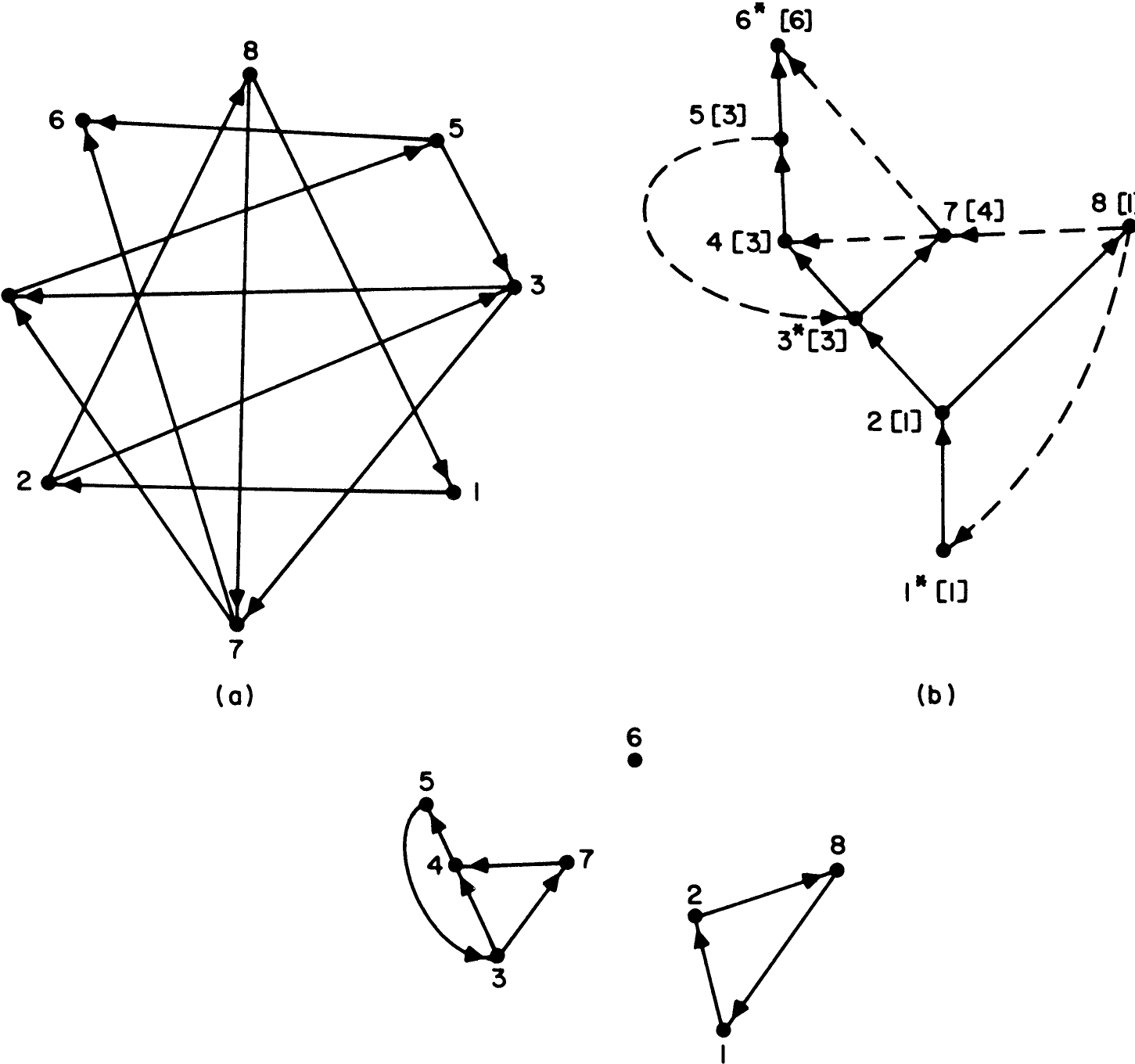
(a) Graph (b) Jungle generated by depth-first search with LOWLINK values in [ ], roots of components marked with * (c) Strongly connected components points once, and each point is removed from the stack of points once. Testing to see if a vertex is on the point stack can be done in a fixed time if a Boolean array is kept which answers this question for each vertex. The amount of extra time required by these operations is linear in $V$ and $E$. Thus STRONGCONNECT has a time bound linear in $V$ and $E$.

Theorem 14. The algorithm for finding strongly connected components works correctly on any directed graph G.

Proof. We prove by induction that the calculation of LOWLINK ($v$) is correct. Suppose as the induction hypothesis that for all vertices $v$ such that $v$ is a proper descendant of vertex $k$ or $v < k$, LOWLINK ($v$) is computed correctly. This means that the test to determine if $v$ is the root of a component is performed correctly for all such vertices $v$. The reader may verify that this somewhat strange induction hypothesis corresponds to considering vertices in the order they are examined for the last time during the depth-first search process.

Consider vertex $v = k$. Let $v \rightarrow^* w_1$ and let $w_1 \rightarrow w_2$ be a vine or cross-link such that $w_2 < v$. If vertices $v$ and $w_2$ have no common ancestor, then before vertex $v$ is reached during the search, vertex $w_2$ must have been removed from the stack of points and placed in a component. (The smallest numbered ancestor of vertex $w_2$ must be a component root.) Thus edge $w_1 \rightarrow w_2$ does not enter into the calculation of LOWLINK ($v$).

Otherwise, let $u$ be the highest common ancestor of $v$ and $w_2$. Vertex $v$ is also the highest common ancestor of $w_1$ and $w_2$. If $u$ is not in the same strongly connected component as $w_2$, then there must be a strongly connected component root on the tree path $u \rightarrow^* w_2$. Since $w_2 < v$, this root was discovered and $w_2$ was removed from the stack of points and placed in a component before the edge $w_1 \rightarrow w_2$ is traversed during the search. Thus $w_1 \rightarrow w_2$ will not enter into the calculation of LOWLINK ($v$). (This can only happen if $w_1 \rightarrow w_2$ is a cross-link.) On the other hand, if $u$ is in the same strongly connected component as $w_2$, there is no component root $r \rightarrow = u$ on the branch $u \rightarrow^* w_2$, and $v \rightarrow w_2$ will be used to calculate LOWLINK ($w_2$), and also LOWLINK ($v$), as desired. Thus LOWLINK ($v$) is calculated correctly, and by induction LOWLINK is calculated correctly for all vertices.

Since the algorithm correctly calculates LOWLINK, it correctly identifies the roots of the strongly connected components. If such a root $u$ is found, the corresponding component contains all the descendants of $u$ which are on the stack of points when $u$ is discovered. These vertices are all on top of the stack of points, and are all put into a component by STRONGCONNECT. Thus STRONGCONNECT works correctly.

1. Further applications. We have seen how the depth-first search method may be used in the construction of very efficient graph algorithms. The two algorithms presented here are in fact optimal to within a constant factor, since every edge and vertex of a graph must be examined to determine a solution to one of the problems. (Given a suitable theoretical framework, this statement may be proved rigorously.) The similarity between biconnectivity and strong connectivity revealed by the depth-first search approach is striking. The possible uses of depth-first search are very general, and are certainly not limited to the examples presented. Hopcroft and Tarjan have constructed an algorithm for finding triconnected components in $O(V, E)$ time by extending the biconnectivity algorithm [8]. An algorithm for testing the planarity of a graph in $O(V)$ time [15] is also based on depth-first search. Combining the connectivity algorithms, the planarity algorithm, and an algorithm for testing isomorphism of triconnected planar graphs [7], we may construct an algorithm to test isomorphism of arbitrary planar graphs in $O(V \log V)$ time [8]. Depth-first search is a powerful technique with many applications.