Generative Adversarial Nets
Département d’informatique et de recherche opérationnelle Université de Montréal Montréal, QC H3C 3J7 arXiv:1406.2661v1 [stat.ML] 10 Jun 2014
Abstract
We propose a new framework for estimating generative models via an adversarial process, in which we simultaneously train two models: a generative model that captures the data distribution, and a discriminative model that estimates the probability that a sample came from the training data rather than . The training procedure for is to maximize the probability of making a mistake. This framework corresponds to a minimax two-player game. In the space of arbitrary functions and , a unique solution exists, with recovering the training data distribution and equal to everywhere. In the case where and are defined by multilayer perceptrons, the entire system can be trained with backpropagation. There is no need for any Markov chains or unrolled approximate inference networks during either training or generation of samples. Experiments demonstrate the potential of the framework through qualitative and quantitative evaluation of the generated samples.
Mạng đối kháng sinh (Generative Adversarial Nets)
Ian J. Goodfellow, Jean Pouget-Abadie1, Mehdi Mirza, Bing Xu, David Warde-Farley, Sherjil Ozair2, Aaron Courville, Yoshua Bengio3
Département d’informatique et de recherche opérationnelle Université de Montréal Montréal, QC H3C 3J7 arXiv:1406.2661v1 [stat.ML] 10 Jun 2014
Tóm tắt
Chúng tôi đề xuất một khung mới để ước lượng các mô hình sinh thông qua một quá trình đối kháng, trong đó chúng tôi đồng thời huấn luyện hai mô hình: một mô hình sinh nắm bắt phân phối dữ liệu, và một mô hình phân biệt ước lượng xác suất rằng một mẫu đến từ dữ liệu huấn luyện thay vì từ . Thủ tục huấn luyện cho là cực đại hóa xác suất mắc lỗi. Khung này tương ứng với một trò chơi minimax hai người chơi. Trong không gian của các hàm tùy ý và , tồn tại một nghiệm duy nhất, với khôi phục phân phối dữ liệu huấn luyện và bằng ở mọi nơi. Trong trường hợp và được định nghĩa bởi các perceptron đa lớp, toàn bộ hệ thống có thể được huấn luyện bằng lan truyền ngược. Không cần bất kỳ chuỗi Markov nào hoặc các mạng suy luận xấp xỉ được cuộn lại trong quá trình huấn luyện hoặc sinh mẫu. Các thí nghiệm chứng minh tiềm năng của khung này thông qua đánh giá định tính và định lượng các mẫu được sinh ra.
1 Introduction
1 Giới thiệu
The promise of deep learning is to discover rich, hierarchical models [2] that represent probability distributions over the kinds of data encountered in artificial intelligence applications, such as natural images, audio waveforms containing speech, and symbols in natural language corpora. So far, the most striking successes in deep learning have involved discriminative models, usually those that map a high-dimensional, rich sensory input to a class label [14], [22]. These striking successes have primarily been based on the backpropagation and dropout algorithms, using piecewise linear units [19, 9, 10] which have a particularly well-behaved gradient . Deep generative models have had less of an impact, due to the difficulty of approximating many intractable probabilistic computations that arise in maximum likelihood estimation and related strategies, and due to difficulty of leveraging the benefits of piecewise linear units in the generative context. We propose a new generative model estimation procedure that sidesteps these difficulties.4
Triển vọng của học sâu (deep learning) là khám phá các mô hình phân cấp phong phú [2] biểu diễn các phân phối xác suất trên những loại dữ liệu gặp trong các ứng dụng trí tuệ nhân tạo, như ảnh tự nhiên, dạng sóng âm thanh chứa tiếng nói và các ký hiệu trong ngữ liệu ngôn ngữ tự nhiên. Cho đến nay, những thành công nổi bật nhất của học sâu gắn với các mô hình phân biệt, thường là những mô hình ánh xạ đầu vào cảm giác phong phú, có số chiều cao sang một nhãn lớp [14], [22]. Những thành công nổi bật này chủ yếu dựa trên các thuật toán lan truyền ngược (backpropagation) và dropout, sử dụng các đơn vị tuyến tính từng khúc [19, 9, 10] có gradient với tính chất đặc biệt thuận lợi. Các mô hình sinh sâu có ít ảnh hưởng hơn, do khó xấp xỉ nhiều phép tính xác suất không khả thi về mặt tính toán xuất hiện trong ước lượng hợp lý cực đại và các chiến lược liên quan, cũng như do khó khai thác lợi ích của các đơn vị tuyến tính từng khúc trong bối cảnh sinh dữ liệu. Chúng tôi đề xuất một thủ tục ước lượng mô hình sinh mới tránh được những khó khăn này.4
In the proposed adversarial nets framework, the generative model is pitted against an adversary: a discriminative model that learns to determine whether a sample is from the model distribution or the data distribution. The generative model can be thought of as analogous to a team of counterfeiters, trying to produce fake currency and use it without detection, while the discriminative model is analogous to the police, trying to detect the counterfeit currency. Competition in this game drives both teams to improve their methods until the counterfeits are indistinguishable from the genuine articles.
Trong khung mạng đối kháng (adversarial nets) được đề xuất, mô hình sinh được đặt vào thế đối đầu với một đối thủ: một mô hình phân biệt học cách xác định một mẫu đến từ phân phối của mô hình hay phân phối dữ liệu. Có thể hình dung mô hình sinh tương tự như một nhóm làm tiền giả, cố gắng tạo ra tiền giả và sử dụng mà không bị phát hiện, trong khi mô hình phân biệt tương tự như cảnh sát, cố gắng phát hiện tiền giả. Sự cạnh tranh trong trò chơi này thúc đẩy cả hai nhóm cải tiến phương pháp của mình cho đến khi không thể phân biệt tiền giả với tiền thật.
This framework can yield specific training algorithms for many kinds of model and optimization algorithm. In this article, we explore the special case when the generative model generates samples by passing random noise through a multilayer perceptron, and the discriminative model is also a multilayer perceptron. We refer to this special case as adversarial nets. In this case, we can train both models using only the highly successful backpropagation and dropout algorithms [17] and sample from the generative model using only forward propagation. No approximate inference or Markov chains are necessary.
Khung này có thể tạo ra các thuật toán huấn luyện cụ thể cho nhiều loại mô hình và thuật toán tối ưu hóa. Trong bài báo này, chúng tôi khảo sát trường hợp đặc biệt khi mô hình sinh tạo các mẫu bằng cách truyền nhiễu ngẫu nhiên qua một perceptron nhiều lớp, và mô hình phân biệt cũng là một perceptron nhiều lớp. Chúng tôi gọi trường hợp đặc biệt này là mạng đối kháng. Trong trường hợp này, chúng tôi có thể huấn luyện cả hai mô hình chỉ bằng các thuật toán lan truyền ngược và dropout vốn rất thành công [17], đồng thời lấy mẫu từ mô hình sinh chỉ bằng lan truyền xuôi. Không cần suy luận xấp xỉ hay chuỗi Markov.
2 Related work
2 Công trình liên quan
An alternative to directed graphical models with latent variables are undirected graphical models with latent variables, such as restricted Boltzmann machines (RBMs) [27, 16], deep Boltzmann machines (DBMs) [26] and their numerous variants. The interactions within such models are represented as the product of unnormalized potential functions, normalized by a global summation/integration over all states of the random variables. This quantity (the partition function) and its gradient are intractable for all but the most trivial instances, although they can be estimated by Markov chain Monte Carlo (MCMC) methods. Mixing poses a significant problem for learning algorithms that rely on MCMC [3, 5].
Một phương án thay thế cho các mô hình đồ thị có hướng với các biến ẩn là các mô hình đồ thị vô hướng với các biến ẩn, chẳng hạn như restricted Boltzmann machines (RBMs) [27, 16], deep Boltzmann machines (DBMs) [26] và nhiều biến thể của chúng. Các tương tác bên trong những mô hình như vậy được biểu diễn dưới dạng tích của các hàm thế chưa chuẩn hóa, được chuẩn hóa bởi một phép tổng/tích phân toàn cục trên tất cả các trạng thái của các biến ngẫu nhiên. Đại lượng này (hàm phân hoạch) và gradient của nó là không thể tính toán được đối với tất cả các trường hợp ngoài những trường hợp tầm thường nhất, mặc dù chúng có thể được ước lượng bằng các phương pháp Markov chain Monte Carlo (MCMC). Việc trộn tạo ra một vấn đề đáng kể đối với các thuật toán học dựa vào MCMC [3, 5].
Deep belief networks (DBNs) [16] are hybrid models containing a single undirected layer and several directed layers. While a fast approximate layer-wise training criterion exists, DBNs incur the computational difficulties associated with both undirected and directed models.
Deep belief networks (DBNs) [16] là các mô hình lai chứa một lớp vô hướng duy nhất và một số lớp có hướng. Mặc dù tồn tại một tiêu chuẩn huấn luyện xấp xỉ nhanh theo từng lớp, DBNs phải chịu các khó khăn về tính toán liên quan đến cả mô hình vô hướng và mô hình có hướng.
Alternative criteria that do not approximate or bound the log-likelihood have also been proposed, such as score matching [18] and noise-contrastive estimation (NCE) [13]. Both of these require the learned probability density to be analytically specified up to a normalization constant. Note that in many interesting generative models with several layers of latent variables (such as DBNs and DBMs), it is not even possible to derive a tractable unnormalized probability density. Some models such as denoising auto-encoders [30] and contractive autoencoders have learning rules very similar to score matching applied to RBMs. In NCE, as in this work, a discriminative training criterion is employed to fit a generative model. However, rather than fitting a separate discriminative model, the generative model itself is used to discriminate generated data from samples a fixed noise distribution. Because NCE uses a fixed noise distribution, learning slows dramatically after the model has learned even an approximately correct distribution over a small subset of the observed variables.
Các tiêu chuẩn thay thế không xấp xỉ hoặc chặn log-likelihood cũng đã được đề xuất, chẳng hạn như score matching [18] và noise-contrastive estimation (NCE) [13]. Cả hai phương pháp này đều yêu cầu mật độ xác suất đã học được đặc tả về mặt giải tích đến một hằng số chuẩn hóa. Lưu ý rằng trong nhiều mô hình sinh thú vị với nhiều lớp biến ẩn (chẳng hạn như DBNs và DBMs), thậm chí không thể suy ra một mật độ xác suất chưa chuẩn hóa có thể tính toán được. Một số mô hình như denoising auto-encoders [30] và contractive autoencoders có các quy tắc học rất giống với score matching được áp dụng cho RBMs. Trong NCE, cũng như trong công trình này, một tiêu chuẩn huấn luyện phân biệt được sử dụng để khớp một mô hình sinh. Tuy nhiên, thay vì khớp một mô hình phân biệt riêng biệt, chính mô hình sinh được dùng để phân biệt dữ liệu được sinh ra với các mẫu từ một phân phối nhiễu cố định. Vì NCE sử dụng một phân phối nhiễu cố định, việc học chậm đi đáng kể sau khi mô hình đã học được ngay cả một phân phối gần đúng chính xác trên một tập con nhỏ của các biến quan sát.
Finally, some techniques do not involve defining a probability distribution explicitly, but rather train a generative machine to draw samples from the desired distribution. This approach has the advantage that such machines can be designed to be trained by back-propagation. Prominent recent work in this area includes the generative stochastic network (GSN) framework [5], which extends generalized denoising auto-encoders [4]: both can be seen as defining a parameterized Markov chain, i.e., one learns the parameters of a machine that performs one step of a generative Markov chain. Compared to GSNs, the adversarial nets framework does not require a Markov chain for sampling. Because adversarial nets do not require feedback loops during generation, they are better able to leverage piecewise linear units [19, 9, 10], which improve the performance of backpropagation but have problems with unbounded activation when used in a feedback loop. More recent examples of training a generative machine by back-propagating into it include recent work on auto-encoding variational Bayes [20] and stochastic backpropagation [24].
Cuối cùng, một số kỹ thuật không liên quan đến việc định nghĩa rõ ràng một phân phối xác suất, mà thay vào đó huấn luyện một máy sinh để lấy các mẫu từ phân phối mong muốn. Phương pháp này có ưu điểm là các máy như vậy có thể được thiết kế để được huấn luyện bằng back-propagation. Các công trình gần đây nổi bật trong lĩnh vực này bao gồm khung generative stochastic network (GSN) [5], mở rộng các denoising auto-encoders tổng quát [4]: cả hai có thể được xem như định nghĩa một chuỗi Markov được tham số hóa, tức là người ta học các tham số của một máy thực hiện một bước của một chuỗi Markov sinh. So với GSN, khung adversarial nets không yêu cầu một chuỗi Markov để lấy mẫu. Vì adversarial nets không yêu cầu các vòng lặp phản hồi trong quá trình sinh, chúng có khả năng tận dụng tốt hơn các đơn vị tuyến tính từng phần [19, 9, 10], vốn cải thiện hiệu năng của backpropagation nhưng gặp vấn đề với kích hoạt không bị chặn khi được sử dụng trong một vòng lặp phản hồi. Các ví dụ gần đây hơn về việc huấn luyện một máy sinh bằng cách lan truyền ngược vào nó bao gồm các công trình gần đây về auto-encoding variational Bayes [20] và stochastic backpropagation [24].
3 Adversarial nets
3 Mạng đối kháng
The adversarial modeling framework is most straightforward to apply when the models are both multilayer perceptrons. To learn the generator’s distribution over data , we define a prior on input noise variables , then represent a mapping to data space as , where is a differentiable function represented by a multilayer perceptron with parameters . We also define a second multilayer perceptron that outputs a single scalar. represents the probability that came from the data rather than . We train to maximize the probability of assigning the correct label to both training examples and samples from . We simultaneously train to minimize :
Khung mô hình hóa đối kháng (adversarial modeling) dễ áp dụng nhất khi cả hai mô hình đều là perceptron đa lớp (multilayer perceptron). Để học phân phối của bộ sinh trên dữ liệu , chúng tôi định nghĩa một phân phối tiên nghiệm trên các biến nhiễu đầu vào , sau đó biểu diễn một ánh xạ tới không gian dữ liệu dưới dạng , trong đó là một hàm khả vi được biểu diễn bằng một perceptron đa lớp có các tham số . Chúng tôi cũng định nghĩa một perceptron đa lớp thứ hai xuất ra một giá trị vô hướng duy nhất. biểu diễn xác suất đến từ dữ liệu thay vì từ . Chúng tôi huấn luyện để tối đa hóa xác suất gán nhãn đúng cho cả các ví dụ huấn luyện lẫn các mẫu từ . Đồng thời, chúng tôi huấn luyện để tối thiểu hóa :
In other words, and play the following two-player minimax game with value function :
Nói cách khác, và tham gia trò chơi minimax hai người chơi sau đây với hàm giá trị :
In the next section, we present a theoretical analysis of adversarial nets, essentially showing that the training criterion allows one to recover the data generating distribution as and are given enough capacity, i.e., in the non-parametric limit. See Figure 1 for a less formal, more pedagogical explanation of the approach. In practice, we must implement the game using an iterative, numerical approach. Optimizing to completion in the inner loop of training is computationally prohibitive, and on finite datasets would result in overfitting. Instead, we alternate between steps of optimizing and one step of optimizing . This results in being maintained near its optimal solution, so long as changes slowly enough. This strategy is analogous to the way that SML/PCD [31, 29] training maintains samples from a Markov chain from one learning step to the next in order to avoid burning in a Markov chain as part of the inner loop of learning. The procedure is formally presented in Algorithm 1.
Trong phần tiếp theo, chúng tôi trình bày một phân tích lý thuyết về mạng đối kháng, về cơ bản cho thấy tiêu chí huấn luyện cho phép khôi phục phân phối sinh dữ liệu khi và có đủ năng lực biểu diễn, tức là trong giới hạn phi tham số. Xem Hình 1 để có cách giải thích ít hình thức hơn và mang tính sư phạm hơn về phương pháp này. Trong thực tế, chúng tôi phải triển khai trò chơi bằng một phương pháp số có tính lặp. Việc tối ưu hóa đến khi hoàn tất trong vòng lặp bên trong của quá trình huấn luyện đòi hỏi chi phí tính toán quá lớn, và trên các tập dữ liệu hữu hạn sẽ dẫn đến quá khớp (overfitting). Thay vào đó, chúng tôi luân phiên thực hiện bước tối ưu hóa và một bước tối ưu hóa . Nhờ vậy, được duy trì gần nghiệm tối ưu của nó, miễn là thay đổi đủ chậm. Chiến lược này tương tự cách quá trình huấn luyện SML/PCD [31, 29] duy trì các mẫu từ một chuỗi Markov từ bước học này sang bước học tiếp theo nhằm tránh phải thực hiện giai đoạn khởi động của chuỗi Markov trong vòng lặp bên trong của quá trình học. Thủ tục này được trình bày một cách hình thức trong Thuật toán 1.
In practice, equation 1 may not provide sufficient gradient for to learn well. Early in learning, when is poor, can reject samples with high confidence because they are clearly different from the training data. In this case, saturates. Rather than training to minimize we can train to maximize . This objective function results in the same fixed point of the dynamics of and but provides much stronger gradients early in learning.
Trong thực tế, phương trình 1 có thể không cung cấp đủ gradient để học tốt. Ở giai đoạn đầu của quá trình học, khi còn kém, có thể bác bỏ các mẫu với độ tin cậy cao vì chúng rõ ràng khác với dữ liệu huấn luyện. Trong trường hợp này, bão hòa. Thay vì huấn luyện để tối thiểu hóa , chúng tôi có thể huấn luyện để tối đa hóa . Hàm mục tiêu này dẫn đến cùng một điểm bất động của động lực học của và nhưng cung cấp các gradient mạnh hơn nhiều ở giai đoạn đầu của quá trình học.
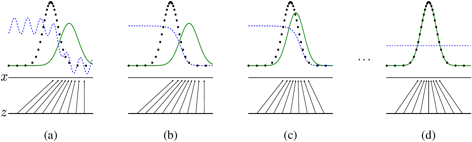
4 Theoretical Results
4 Các kết quả lý thuyết
The generator implicitly defines a probability distribution as the distribution of the samples obtained when . Therefore, we would like Algorithm 1 to converge to a good estimator of , if given enough capacity and training time. The results of this section are done in a non-parametric setting, e.g. we represent a model with infinite capacity by studying convergence in the space of probability density functions.
Bộ sinh định nghĩa một cách ngầm định một phân phối xác suất như là phân phối của các mẫu thu được khi . Do đó, chúng tôi muốn Algorithm 1 hội tụ đến một bộ ước lượng tốt của , nếu được cung cấp đủ năng lực và thời gian huấn luyện. Các kết quả của phần này được thực hiện trong thiết lập phi tham số, ví dụ, chúng tôi biểu diễn một mô hình với năng lực vô hạn bằng cách nghiên cứu sự hội tụ trong không gian của các hàm mật độ xác suất.
We will show in section 4.1 that this minimax game has a global optimum for . We will then show in section 4.2 that Algorithm 1 optimizes Eq 1, thus obtaining the desired result.
Chúng tôi sẽ chỉ ra trong phần 4.1 rằng trò chơi minimax này có một cực trị toàn cục cho . Sau đó, chúng tôi sẽ chỉ ra trong phần 4.2 rằng Algorithm 1 tối ưu hóa Eq 1, do đó thu được kết quả mong muốn.
Algorithm 1 Minibatch stochastic gradient descent training of generative adversarial nets. The number of steps to apply to the discriminator, , is a hyperparameter. We used , the least expensive option in our experiments.
Algorithm 1 Huấn luyện giảm gradient ngẫu nhiên theo lô nhỏ của các mạng đối kháng sinh. Số bước áp dụng cho bộ phân biệt, , là một siêu tham số. Chúng tôi sử dụng , tùy chọn ít tốn kém nhất trong các thí nghiệm của mình.
for number of training iterations do
for số lần lặp huấn luyện do
for steps do
for bước do
- Sample minibatch of noise samples from noise prior .
- Sample minibatch of examples from data generating distribution .
- Update the discriminator by ascending its stochastic gradient:
- Lấy mẫu lô nhỏ gồm mẫu nhiễu từ tiên nghiệm nhiễu .
- Lấy mẫu lô nhỏ gồm ví dụ từ phân phối sinh dữ liệu .
- Cập nhật bộ phân biệt bằng cách tăng gradient ngẫu nhiên của nó:
end for
end for
- Sample minibatch of noise samples from noise prior .
- Update the generator by descending its stochastic gradient:
- Lấy mẫu lô nhỏ gồm mẫu nhiễu từ tiên nghiệm nhiễu .
- Cập nhật bộ sinh bằng cách giảm gradient ngẫu nhiên của nó:
end for
end for
The gradient-based updates can use any standard gradient-based learning rule. We used momentum in our experiments.
Các cập nhật dựa trên gradient có thể sử dụng bất kỳ quy tắc học dựa trên gradient tiêu chuẩn nào. Chúng tôi đã sử dụng động lượng trong các thí nghiệm của mình.
4.1 Global Optimality of
4.1 Tính tối ưu toàn cục của
We first consider the optimal discriminator for any given generator .
Trước tiên chúng tôi xét bộ phân biệt tối ưu đối với bất kỳ bộ sinh đã cho nào.
Proposition 1. For fixed, the optimal discriminator is
Proposition 1. Với cố định, bộ phân biệt tối ưu là
Proof. The training criterion for the discriminator D, given any generator G, is to maximize the quantity
Proof. Tiêu chuẩn huấn luyện cho bộ phân biệt D, với bất kỳ bộ sinh G nào, là cực đại hóa đại lượng
For any , the function achieves its maximum in at . The discriminator does not need to be defined outside of , concluding the proof.
Với mọi , hàm đạt giá trị cực đại trong tại . Bộ phân biệt không cần được định nghĩa bên ngoài , hoàn tất chứng minh.
Note that the training objective for can be interpreted as maximizing the log-likelihood for estimating the conditional probability , where indicates whether comes from (with ) or from (with ). The minimax game in Eq. 1 can now be reformulated as:
Lưu ý rằng mục tiêu huấn luyện cho có thể được diễn giải như việc cực đại hóa log-likelihood để ước lượng xác suất có điều kiện , trong đó chỉ ra liệu đến từ (với ) hay từ (với ). Trò chơi minimax trong Eq. 1 giờ đây có thể được viết lại thành:
Theorem 1. The global minimum of the virtual training criterion is achieved if and only if . At that point, achieves the value .
Theorem 1. Cực tiểu toàn cục của tiêu chuẩn huấn luyện ảo đạt được khi và chỉ khi . Tại điểm đó, đạt giá trị .
Proof. For , , (consider Eq. 2). Hence, by inspecting Eq. 4 at , we find . To see that this is the best possible value of , reached only for , observe that
Proof. Với , , (xét Eq. 2). Do đó, bằng cách kiểm tra Eq. 4 tại , chúng ta nhận thấy . Để thấy rằng đây là giá trị tốt nhất có thể của , chỉ đạt được khi , hãy quan sát rằng
and that by subtracting this expression from , we obtain:
và bằng cách trừ biểu thức này khỏi , ta thu được:
where KL is the Kullback–Leibler divergence. We recognize in the previous expression the Jensen–Shannon divergence between the model’s distribution and the data generating process:
trong đó KL là độ phân kỳ Kullback–Leibler. Chúng ta nhận ra trong biểu thức trước đó độ phân kỳ Jensen–Shannon giữa phân phối của mô hình và quá trình sinh dữ liệu:
Since the Jensen–Shannon divergence between two distributions is always non-negative and zero only when they are equal, we have shown that is the global minimum of and that the only solution is , i.e., the generative model perfectly replicating the data generating process.
Vì độ phân kỳ Jensen–Shannon giữa hai phân phối luôn không âm và bằng không chỉ khi chúng bằng nhau, chúng ta đã chứng minh rằng là cực tiểu toàn cục của và nghiệm duy nhất là , tức là mô hình sinh sao chép hoàn hảo quá trình sinh dữ liệu.
4.2 Convergence of Algorithm 1
4.2 Sự hội tụ của Thuật toán 1
Proposition 2. If and have enough capacity, and at each step of Algorithm 1, the discriminator is allowed to reach its optimum given , and is updated so as to improve the criterion
Mệnh đề 2. Nếu và có đủ năng lực, và tại mỗi bước của Thuật toán 1, bộ phân biệt được phép đạt đến tối ưu của nó với đã cho, và được cập nhật để cải thiện tiêu chí
then converges to
thì hội tụ về
Proof. Consider as a function of as done in the above criterion. Note that is convex in . The subderivatives of a supremum of convex functions include the derivative of the function at the point where the maximum is attained. In other words, if and is convex in for every , then if . This is equivalent to computing a gradient descent update for at the optimal given the corresponding . is convex in with a unique global optima as proven in Thm 1, therefore with sufficiently small updates of , converges to , concluding the proof.
Chứng minh. Xét như một hàm của giống như đã thực hiện trong tiêu chí ở trên. Lưu ý rằng là lồi theo . Các đạo hàm con của một supremum của các hàm lồi bao gồm đạo hàm của hàm tại điểm đạt được giá trị cực đại. Nói cách khác, nếu và là lồi theo với mọi , thì nếu . Điều này tương đương với việc tính một cập nhật gradient descent cho tại tối ưu ứng với tương ứng. là lồi theo với một tối ưu toàn cục duy nhất như đã được chứng minh trong Định lý 1, do đó với các cập nhật đủ nhỏ, hội tụ về , hoàn tất chứng minh.
In practice, adversarial nets represent a limited family of distributions via the function , and we optimize rather than itself. Using a multilayer perceptron to define introduces multiple critical points in parameter space. However, the excellent performance of multilayer perceptrons in practice suggests that they are a reasonable model to use despite their lack of theoretical guarantees.
Trong thực tế, các mạng đối nghịch biểu diễn một họ giới hạn các phân phối thông qua hàm , và chúng tôi tối ưu hóa thay vì bản thân . Việc sử dụng một perceptron đa lớp để định nghĩa đưa vào nhiều điểm tới hạn trong không gian tham số. Tuy nhiên, hiệu năng xuất sắc của các perceptron đa lớp trong thực tế cho thấy chúng là một mô hình hợp lý để sử dụng mặc dù thiếu các đảm bảo lý thuyết.
5 Experiments
5 Thực nghiệm
We trained adversarial nets on a range of datasets including MNIST[23], the Toronto Face Database (TFD) [28], and CIFAR-10 [21]. The generator nets used a mixture of rectifier linear activations [19, 9] and sigmoid activations, while the discriminator net used maxout [10] activations. Dropout [17] was applied in training the discriminator net. While our theoretical framework permits the use of dropout and other noise at intermediate layers of the generator, we used noise as the input to only the bottommost layer of the generator network.
Chúng tôi đã huấn luyện các mạng đối kháng (adversarial nets) trên nhiều tập dữ liệu, bao gồm MNIST[23], Toronto Face Database (TFD) [28] và CIFAR-10 [21]. Các mạng sinh sử dụng kết hợp các hàm kích hoạt tuyến tính chỉnh lưu [19, 9] và các hàm kích hoạt sigmoid, trong khi mạng phân biệt sử dụng các hàm kích hoạt maxout [10]. Dropout [17] được áp dụng khi huấn luyện mạng phân biệt. Mặc dù khung lý thuyết của chúng tôi cho phép sử dụng dropout và các dạng nhiễu khác tại các lớp trung gian của bộ sinh, chúng tôi chỉ đưa nhiễu vào lớp dưới cùng của mạng sinh.
We estimate probability of the test set data under by fitting a Gaussian Parzen window to the samples generated with and reporting the log-likelihood under this distribution. The parameter
Chúng tôi ước lượng xác suất của dữ liệu tập kiểm thử theo bằng cách khớp một cửa sổ Parzen Gauss với các mẫu được sinh bằng và báo cáo log hợp lý (log-likelihood) theo phân phối này. Tham số
Table 1: Parzen window-based log-likelihood estimates. The reported numbers on MNIST are the mean log-likelihood of samples on test set, with the standard error of the mean computed across examples. On TFD, we computed the standard error across folds of the dataset, with a different chosen using the validation set of each fold. On TFD, was cross validated on each fold and mean log-likelihood on each fold were computed. For MNIST we compare against other models of the real-valued (rather than binary) version of dataset.
Bảng 1: Các ước lượng log hợp lý dựa trên cửa sổ Parzen. Các số được báo cáo trên MNIST là log hợp lý trung bình của các mẫu trong tập kiểm thử, với sai số chuẩn của trung bình được tính trên các mẫu. Trên TFD, chúng tôi tính sai số chuẩn trên các phần chia của tập dữ liệu, với một khác nhau được chọn bằng tập thẩm định của từng phần chia. Trên TFD, được thẩm định chéo trên từng phần chia và log hợp lý trung bình trên từng phần chia được tính toán. Với MNIST, chúng tôi so sánh với các mô hình khác trên phiên bản có giá trị thực (thay vì nhị phân) của tập dữ liệu.
of the Gaussians was obtained by cross validation on the validation set. This procedure was introduced in Breuleux et al. [8] and used for various generative models for which the exact likelihood is not tractable [25, 3, 5]. Results are reported in Table 1. This method of estimating the likelihood has somewhat high variance and does not perform well in high dimensional spaces but it is the best method available to our knowledge. Advances in generative models that can sample but not estimate likelihood directly motivate further research on how to evaluate such models.
của các phân phối Gauss được xác định bằng thẩm định chéo trên tập thẩm định. Thủ tục này được giới thiệu bởi Breuleux và cộng sự [8] và được sử dụng cho nhiều mô hình sinh mà việc tính chính xác hợp lý là bất khả thi [25, 3, 5]. Kết quả được báo cáo trong Bảng 1. Phương pháp ước lượng hợp lý này có phương sai tương đối cao và hoạt động không tốt trong các không gian nhiều chiều, nhưng theo hiểu biết của chúng tôi, đây là phương pháp tốt nhất hiện có. Những tiến bộ trong các mô hình sinh có thể lấy mẫu nhưng không thể trực tiếp ước lượng hợp lý thúc đẩy việc nghiên cứu thêm về cách đánh giá các mô hình như vậy.
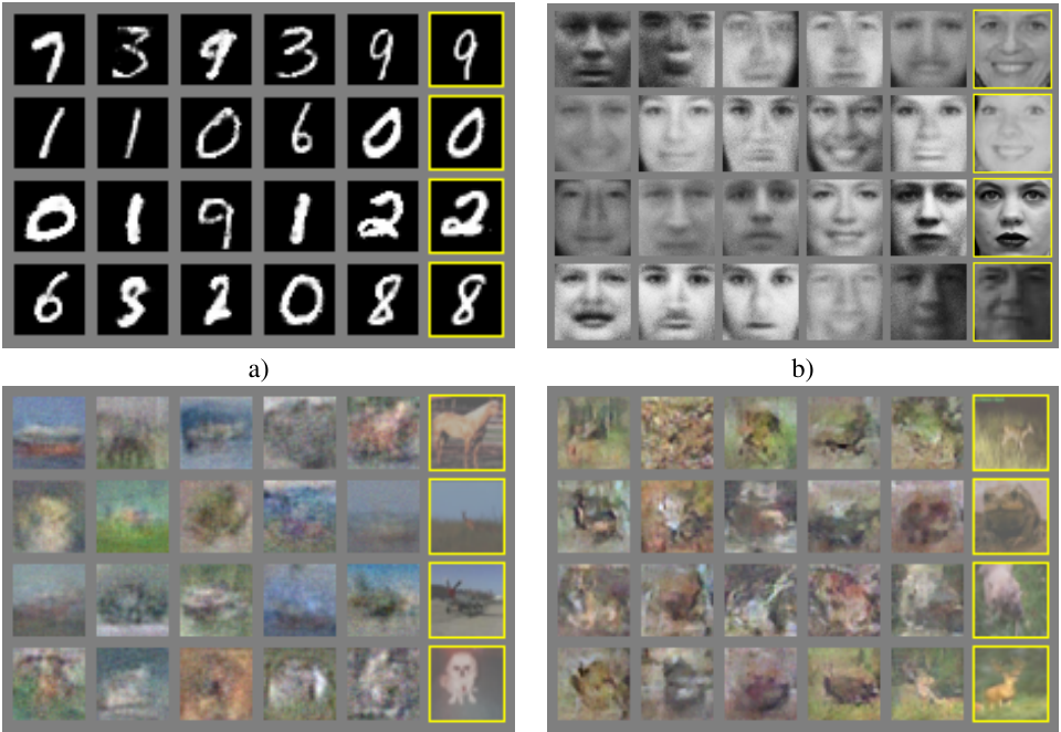
In Figures 2 and 3 we show samples drawn from the generator net after training. While we make no claim that these samples are better than samples generated by existing methods, we believe that these samples are at least competitive with the better generative models in the literature and highlight the potential of the adversarial framework.
Trong Hình 2 và 3, chúng tôi trình bày các mẫu được lấy từ mạng sinh sau khi huấn luyện. Mặc dù chúng tôi không khẳng định rằng các mẫu này tốt hơn các mẫu được sinh bằng những phương pháp hiện có, chúng tôi tin rằng các mẫu này ít nhất có thể cạnh tranh với các mô hình sinh tốt hơn trong tài liệu nghiên cứu và cho thấy tiềm năng của khung đối kháng.

| Deep directed graphical models | Deep undirected graphical models | Generative autoencoders | Adversarial models | |
|---|---|---|---|---|
| Training | Inference needed during training. | Inference needed during training. MCMC needed to approximate partition function gradient. | Enforced tradeoff between mixing and power of reconstruction generation | Synchronizing the discriminator with the generator. Helvetica. |
| Inference | Learned approximate inference | Variational inference | MCMC-based inference | Learned approximate inference |
| Sampling | No difficulties | Requires Markov chain | Requires Markov chain | No difficulties |
| Evaluating | Intractable, may be approximated with AIS | Intractable, may be approximated with AIS | Not explicitly represented, may be approximated with Parzen density estimation | Not explicitly represented, may be approximated with Parzen density estimation |
| Model design | Nearly all models incur extreme difficulty | Careful design needed to ensure multiple properties | Any differentiable function is theoretically permitted | Any differentiable function is theoretically permitted |
| Mô hình đồ thị có hướng sâu | Mô hình đồ thị vô hướng sâu | Bộ tự mã hóa sinh | Mô hình đối kháng | |
|---|---|---|---|---|
| Huấn luyện | Cần suy luận trong quá trình huấn luyện. | Cần suy luận trong quá trình huấn luyện. Cần MCMC để xấp xỉ gradient của hàm phân hoạch. | Buộc phải đánh đổi giữa sự trộn và khả năng sinh tái tạo | Đồng bộ hóa bộ phân biệt với bộ sinh. Helvetica. |
| Suy luận | Suy luận xấp xỉ được học | Suy luận biến phân | Suy luận dựa trên MCMC | Suy luận xấp xỉ được học |
| Lấy mẫu | Không có khó khăn | Cần chuỗi Markov | Cần chuỗi Markov | Không có khó khăn |
| Đánh giá | Không thể tính toán khả thi, có thể xấp xỉ bằng AIS | Không thể tính toán khả thi, có thể xấp xỉ bằng AIS | Không được biểu diễn tường minh, có thể xấp xỉ bằng ước lượng mật độ Parzen | Không được biểu diễn tường minh, có thể xấp xỉ bằng ước lượng mật độ Parzen |
| Thiết kế mô hình | Gần như mọi mô hình đều gặp khó khăn cực lớn | Cần thiết kế cẩn thận để bảo đảm nhiều tính chất | Về lý thuyết, cho phép mọi hàm khả vi | Về lý thuyết, cho phép mọi hàm khả vi |
Table 2: Challenges in generative modeling: a summary of the difficulties encountered by different approaches to deep generative modeling for each of the major operations involving a model.
Bảng 2: Những thách thức trong mô hình hóa sinh: tóm tắt các khó khăn mà những cách tiếp cận khác nhau đối với mô hình hóa sinh sâu gặp phải trong từng thao tác chính liên quan đến một mô hình.
6 Advantages and disadvantages
6 Ưu điểm và nhược điểm
This new framework comes with advantages and disadvantages relative to previous modeling frameworks. The disadvantages are primarily that there is no explicit representation of , and that must be synchronized well with during training (in particular, must not be trained too much without updating , in order to avoid “the Helvetica scenario” in which collapses too many values of to the same value of to have enough diversity to model ), much as the negative chains of a Boltzmann machine must be kept up to date between learning steps. The advantages are that Markov chains are never needed, only backprop is used to obtain gradients, no inference is needed during learning, and a wide variety of functions can be incorporated into the model. Table 2 summarizes the comparison of generative adversarial nets with other generative modeling approaches.
Khung mới này đi kèm với các ưu điểm và nhược điểm so với các khung mô hình hóa trước đây. Các nhược điểm chủ yếu là không có biểu diễn tường minh của , và phải được đồng bộ tốt với trong quá trình huấn luyện (đặc biệt, không được huấn luyện quá nhiều mà không cập nhật , nhằm tránh “kịch bản Helvetica”, trong đó thu gọn quá nhiều giá trị của thành cùng một giá trị của đến mức không có đủ tính đa dạng để mô hình hóa ), tương tự như các chuỗi âm của máy Boltzmann phải được cập nhật kịp thời giữa các bước học. Các ưu điểm là không bao giờ cần đến các chuỗi Markov, chỉ sử dụng backprop để thu được các gradient, không cần suy luận trong quá trình học, và có thể tích hợp nhiều loại hàm vào mô hình. Bảng 2 tóm tắt sự so sánh giữa các mạng đối nghịch sinh và các phương pháp mô hình hóa sinh khác.
The aforementioned advantages are primarily computational. Adversarial models may also gain some statistical advantage from the generator network not being updated directly with data examples, but only with gradients flowing through the discriminator. This means that components of the input are not copied directly into the generator’s parameters. Another advantage of adversarial networks is that they can represent very sharp, even degenerate distributions, while methods based on Markov chains require that the distribution be somewhat blurry in order for the chains to be able to mix between modes.
Các ưu điểm nêu trên chủ yếu mang tính toán học. Các mô hình đối nghịch cũng có thể đạt được một số lợi thế thống kê từ việc mạng sinh không được cập nhật trực tiếp bằng các ví dụ dữ liệu, mà chỉ bằng các gradient truyền qua bộ phân biệt. Điều này có nghĩa là các thành phần của đầu vào không được sao chép trực tiếp vào các tham số của bộ sinh. Một ưu điểm khác của các mạng đối nghịch là chúng có thể biểu diễn các phân phối rất sắc nét, thậm chí suy biến, trong khi các phương pháp dựa trên chuỗi Markov yêu cầu phân phối phải hơi mờ để các chuỗi có thể trộn giữa các mode.
7 Conclusions and future work
7 Kết luận và hướng nghiên cứu tương lai
This framework admits many straightforward extensions:
Khung này cho phép nhiều mở rộng trực tiếp:
- A conditional generative model can be obtained by adding as input to both and .
- Learned approximate inference can be performed by training an auxiliary network to predict given . This is similar to the inference net trained by the wake-sleep algorithm [15] but with the advantage that the inference net may be trained for a fixed generator net after the generator net has finished training.
- Có thể thu được mô hình sinh có điều kiện (conditional generative model) bằng cách thêm làm đầu vào cho cả và .
- Có thể thực hiện suy luận xấp xỉ thông qua học (learned approximate inference) bằng cách huấn luyện một mạng phụ để dự đoán khi biết . Cách này tương tự mạng suy luận được huấn luyện bằng thuật toán wake-sleep [15] nhưng có ưu điểm là mạng suy luận có thể được huấn luyện với một mạng sinh cố định sau khi mạng sinh đã hoàn tất huấn luyện.
- One can approximately model all conditionals where is a subset of the indices of by training a family of conditional models that share parameters. Essentially, one can use adversarial nets to implement a stochastic extension of the deterministic MP-DBM [11].
- Semi-supervised learning: features from the discriminator or inference net could improve performance of classifiers when limited labeled data is available.
- Efficiency improvements: training could be accelerated greatly by divising better methods for coordinating and or determining better distributions to sample from during training.
- Có thể mô hình hóa xấp xỉ tất cả các phân phối có điều kiện , trong đó là một tập con của tập chỉ số của , bằng cách huấn luyện một họ mô hình có điều kiện dùng chung tham số. Về bản chất, có thể dùng các mạng đối kháng để triển khai một mở rộng ngẫu nhiên của MP-DBM tất định [11].
- Học bán giám sát (semi-supervised learning): các đặc trưng từ mạng phân biệt hoặc mạng suy luận có thể cải thiện hiệu năng của các bộ phân loại khi dữ liệu có nhãn còn hạn chế.
- Cải thiện hiệu quả: có thể tăng tốc đáng kể quá trình huấn luyện bằng cách xây dựng các phương pháp tốt hơn để phối hợp và hoặc xác định các phân phối tốt hơn để lấy mẫu trong quá trình huấn luyện.
This paper has demonstrated the viability of the adversarial modeling framework, suggesting that these research directions could prove useful.
Bài báo này đã chứng minh tính khả thi của khung mô hình hóa đối kháng, cho thấy những hướng nghiên cứu này có thể mang lại lợi ích.
Acknowledgments
Lời cảm ơn
We would like to acknowledge Patrice Marcotte, Olivier Delalleau, Kyunghyun Cho, Guillaume Alain and Jason Yosinski for helpful discussions. Yann Dauphin shared his Parzen window evaluation code with us. We would like to thank the developers of Pylearn2 [12] and Theano [7, 1], particularly Frédéric Bastien who shared a Theano feature specifically to benefit this project. Arnaud Bergeron provided much-needed support with typesetting. We would also like to thank CIFAR, and Canada Research Chairs for funding, and Compute Canada, and Calcul Québec for providing computational resources. Ian Goodfellow is supported by the 2013 Google Fellowship in Deep Learning. Finally, we would like to thank Les Trois Brasseurs for stimulating our creativity.
Chúng tôi xin cảm ơn Patrice Marcotte, Olivier Delalleau, Kyunghyun Cho, Guillaume Alain và Jason Yosinski vì những trao đổi hữu ích. Yann Dauphin đã chia sẻ với chúng tôi mã đánh giá bằng cửa sổ Parzen (Parzen window). Chúng tôi xin cảm ơn các nhà phát triển Pylearn2 [12] và Theano [7, 1], đặc biệt là Frédéric Bastien, người đã chia sẻ một đặc trưng của Theano dành riêng cho dự án này. Arnaud Bergeron đã hỗ trợ rất cần thiết trong việc dàn trang bằng . Chúng tôi cũng xin cảm ơn CIFAR và Canada Research Chairs đã tài trợ, cùng Compute Canada và Calcul Québec đã cung cấp tài nguyên tính toán. Ian Goodfellow nhận được hỗ trợ từ học bổng Google năm 2013 về học sâu (Deep Learning). Cuối cùng, chúng tôi xin cảm ơn Les Trois Brasseurs đã khơi gợi sự sáng tạo của chúng tôi.
Notes
- Jean Pouget-Abadie is visiting Université de Montréal from Ecole Polytechnique.
- Sherjil Ozair is visiting Université de Montréal from Indian Institute of Technology Delhi
- Yoshua Bengio is a CIFAR Senior Fellow.
- All code and hyperparameters available at http://www.github.com/goodfeli/adversarial
References
- Bastien, F., Lamblin, P., Pascanu, R., Bergstra, J., Goodfellow, I. J., Bergeron, A., Bouchard, N., and Bengio, Y. (2012). Theano: new features and speed improvements. Deep Learning and Unsupervised Feature Learning NIPS 2012 Workshop.
- Bengio, Y. (2009). *Learning deep architectures for AI.* Now Publishers.
- Bengio, Y., Mesnil, G., Dauphin, Y., and Rifai, S. (2013a). Better mixing via deep representations. In *ICML’13*.
- Bengio, Y., Yao, L., Alain, G., and Vincent, P. (2013b). Generalized denoising auto-encoders as generative models. In *NIPS26*. Nips Foundation.
- Bengio, Y., Thibodeau-Laufer, E., and Yosinski, J. (2014a). Deep generative stochastic networks trainable by backprop. In *ICML’14*.
- Bengio, Y., Thibodeau-Laufer, E., Alain, G., and Yosinski, J. (2014b). Deep generative stochastic networks trainable by backprop. In *Proceedings of the 30th International Conference on Machine Learning (ICML’14)*.
- Bergstra, J., Breuleux, O., Bastien, F., Lamblin, P., Pascanu, R., Desjardins, G., Turian, J., Warde-Farley, D., and Bengio, Y. (2010). Theano: a CPU and GPU math expression compiler. In *Proceedings of the Python for Scientific Computing Conference (SciPy)*. Oral Presentation.
- Breuleux, O., Bengio, Y., and Vincent, P. (2011). Quickly generating representative samples from an RBM-derived process. *Neural Computation*, **23**(8), 2053–2073.
- Glorot, X., Bordes, A., and Bengio, Y. (2011). Deep sparse rectifier neural networks. In *AISTATS’2011*.
- Goodfellow, I. J., Warde-Farley, D., Mirza, M., Courville, A., and Bengio, Y. (2013a). Maxout networks. In *ICML’2013*.
- Goodfellow, I. J., Mirza, M., Courville, A., and Bengio, Y. (2013b). Multi-prediction deep Boltzmann machines. In *NIPS’2013*.
- Goodfellow, I. J., Warde-Farley, D., Lamblin, P., Dumoulin, V., Mirza, M., Pascanu, R., Bergstra, J., Bastien, F., and Bengio, Y. (2013c). Pylearn2: a machine learning research library. *arXiv preprint arXiv:1308.4214*.
- Gutmann, M. and Hyvarinen, A. (2010). Noise-contrastive estimation: A new estimation principle for unnormalized statistical models. In *AISTATS’2010*.
- Hinton, G., Deng, L., Dahl, G. E., Mohamed, A., Jaitly, N., Senior, A., Vanhoucke, V., Nguyen, P., Sainath, T., and Kingsbury, B. (2012a). Deep neural networks for acoustic modeling in speech recognition. *IEEE Signal Processing Magazine*, **29**(6), 82–97.
- Hinton, G. E., Dayan, P., Frey, B. J., and Neal, R. M. (1995). The wake-sleep algorithm for unsupervised neural networks. *Science*, **268**, 1558–1161.
- Hinton, G. E., Osindero, S., and Teh, Y. (2006). A fast learning algorithm for deep belief nets. *Neural Computation*, **18**, 1527–1554.
- Hinton, G. E., Srivastava, N., Krizhevsky, A., Sutskever, I., and Salakhutdinov, R. (2012b). Improving neural networks by preventing co-adaptation of feature detectors. Technical report, arXiv:1207.0580.
- Hyvärinen, A. (2005). Estimation of non-normalized statistical models using score matching. *J. Machine Learning Res.*, **6**.
- Jarrett, K., Kavukcuoglu, K., Ranzato, M., and LeCun, Y. (2009). What is the best multi-stage architecture for object recognition? In *Proc. International Conference on Computer Vision (ICCV’09)*, pages 2146–2153. IEEE.
- Kingma, D. P. and Welling, M. (2014). Auto-encoding variational bayes. In *Proceedings of the International Conference on Learning Representations (ICLR)*.
- Krizhevsky, A. and Hinton, G. (2009). Learning multiple layers of features from tiny images. Technical report, University of Toronto.
- Krizhevsky, A., Sutskever, I., and Hinton, G. (2012). ImageNet classification with deep convolutional neural networks. In *NIPS’2012*. Read it here
- LeCun, Y., Bottou, L., Bengio, Y., and Haffner, P. (1998). Gradient-based learning applied to document recognition. *Proceedings of the IEEE*, **86**(11), 2278–2324. Read it here
- Rezende, D. J., Mohamed, S., and Wierstra, D. (2014). Stochastic backpropagation and approximate inference in deep generative models. Technical report, arXiv:1401.4082.
- Rifai, S., Bengio, Y., Dauphin, Y., and Vincent, P. (2012). A generative process for sampling contractive auto-encoders. In *ICML’12*.
- Salakhutdinov, R. and Hinton, G. E. (2009). Deep Boltzmann machines. In *AISTATS’2009*, pages 448–455.
- Smolensky, P. (1986). Information processing in dynamical systems: Foundations of harmony theory. In D. E. Rumelhart and J. L. McClelland, editors, *Parallel Distributed Processing*, volume 1, chapter 6, pages 194–281. MIT Press, Cambridge.
- Susskind, J., Anderson, A., and Hinton, G. E. (2010). The Toronto face dataset. Technical Report UTML TR 2010-001, U. Toronto.
- Tieleman, T. (2008). Training restricted Boltzmann machines using approximations to the likelihood gradient. In W. W. Cohen, A. McCallum, and S. T. Roweis, editors, *ICML 2008*, pages 1064–1071. ACM.
- Vincent, P., Larochelle, H., Bengio, Y., and Manzagol, P.-A. (2008). Extracting and composing robust features with denoising autoencoders. In *ICML 2008*.
- Younes, L. (1999). On the convergence of Markovian stochastic algorithms with rapidly decreasing ergodicity rates. *Stochastics and Stochastic Reports*, **65**(3), 177–228.
Read off the page by a vision model reading the page images using gpt-6-astra.
Read off the page by a vision model reading the page images using gpt-6-astra. Translated from the English.