Generative Adversarial Nets
生成对抗网络
Ian J. Goodfellow, Jean Pouget-Abadie1, Mehdi Mirza, Bing Xu, David Warde-Farley, Sherjil Ozair2, Aaron Courville, Yoshua Bengio3
Département d’informatique et de recherche opérationnelle Université de Montréal Montréal, QC H3C 3J7
arXiv:1406.2661v1 [stat.ML] 10 Jun 2014
摘要
我们提出了一种通过对抗过程估计生成模型的新框架,在该过程中,我们同时训练两个模型:一个捕获数据分布的生成模型,以及一个判别模型,用于估计样本来自训练数据而非的概率。的训练过程是最大化出错的概率。该框架对应于一个极小极大双人博弈。在任意函数和的空间中,存在唯一解,其中恢复训练数据分布,而处处等于。当和由多层感知机定义时,整个系统可以通过反向传播进行训练。在训练或生成样本的过程中,都不需要任何马尔可夫链或展开的近似推理网络。实验通过对生成样本进行定性和定量评估,展示了该框架的潜力。
Département d’informatique et de recherche opérationnelle Université de Montréal Montréal, QC H3C 3J7 arXiv:1406.2661v1 [stat.ML] 10 Jun 2014
Abstract
We propose a new framework for estimating generative models via an adversarial process, in which we simultaneously train two models: a generative model that captures the data distribution, and a discriminative model that estimates the probability that a sample came from the training data rather than . The training procedure for is to maximize the probability of making a mistake. This framework corresponds to a minimax two-player game. In the space of arbitrary functions and , a unique solution exists, with recovering the training data distribution and equal to everywhere. In the case where and are defined by multilayer perceptrons, the entire system can be trained with backpropagation. There is no need for any Markov chains or unrolled approximate inference networks during either training or generation of samples. Experiments demonstrate the potential of the framework through qualitative and quantitative evaluation of the generated samples.
1 引言
1 Introduction
深度学习的前景在于发现丰富的、层次化的模型[2],这些模型表示人工智能应用中遇到的各类数据上的概率分布,例如自然图像、包含语音的音频波形以及自然语言语料中的符号。到目前为止,深度学习最引人注目的成功主要来自判别模型,通常是那些将高维、丰富的感知输入映射到类别标签的模型[14],[22]。这些显著成功主要建立在反向传播和Dropout算法之上,使用分段线性单元[19, 9, 10],其梯度具有特别良好的性质。深度生成模型的影响则较小,这是由于难以近似最大似然估计及相关策略中出现的许多难以处理的概率计算,也由于难以在生成场景中利用分段线性单元的优势。我们提出一种新的生成模型估计过程,绕开了这些困难。4
The promise of deep learning is to discover rich, hierarchical models [2] that represent probability distributions over the kinds of data encountered in artificial intelligence applications, such as natural images, audio waveforms containing speech, and symbols in natural language corpora. So far, the most striking successes in deep learning have involved discriminative models, usually those that map a high-dimensional, rich sensory input to a class label [14], [22]. These striking successes have primarily been based on the backpropagation and dropout algorithms, using piecewise linear units [19, 9, 10] which have a particularly well-behaved gradient . Deep generative models have had less of an impact, due to the difficulty of approximating many intractable probabilistic computations that arise in maximum likelihood estimation and related strategies, and due to difficulty of leveraging the benefits of piecewise linear units in the generative context. We propose a new generative model estimation procedure that sidesteps these difficulties.4
在所提出的对抗网络框架中,生成模型与一个对手相对抗:一个学习判定样本来自模型分布还是数据分布的判别模型。生成模型可以被看作一群造假者,试图制造并使用假币而不被发现;而判别模型则类似于警察,试图识别假币。这场博弈中的竞争推动双方不断改进各自的方法,直到伪造品与真品无法区分。
In the proposed adversarial nets framework, the generative model is pitted against an adversary: a discriminative model that learns to determine whether a sample is from the model distribution or the data distribution. The generative model can be thought of as analogous to a team of counterfeiters, trying to produce fake currency and use it without detection, while the discriminative model is analogous to the police, trying to detect the counterfeit currency. Competition in this game drives both teams to improve their methods until the counterfeits are indistinguishable from the genuine articles.
该框架能够为多种类型的模型和优化算法导出具体的训练算法。本文探索一种特殊情形:生成模型通过将随机噪声传入多层感知机来生成样本,而判别模型也是一个多层感知机。我们将这一特殊情形称为对抗网络。在这种情况下,我们只需使用极其成功的反向传播和Dropout算法[17]即可训练两个模型,并且只需前向传播即可从生成模型中采样。不需要近似推理或马尔可夫链。
This framework can yield specific training algorithms for many kinds of model and optimization algorithm. In this article, we explore the special case when the generative model generates samples by passing random noise through a multilayer perceptron, and the discriminative model is also a multilayer perceptron. We refer to this special case as adversarial nets. In this case, we can train both models using only the highly successful backpropagation and dropout algorithms [17] and sample from the generative model using only forward propagation. No approximate inference or Markov chains are necessary.
2 相关工作
2 Related work
有潜变量的有向图模型的一种替代方案是有潜变量的无向图模型,例如受限玻尔兹曼机(RBM)[27, 16]、深度玻尔兹曼机(DBM)[26]及其众多变体。这类模型中的相互作用被表示为未归一化势函数乘积的形式,并通过对随机变量所有状态进行全局求和/积分来归一化。这一量(即配分函数)及其梯度除最平凡的情形外都难以处理,不过可以通过马尔可夫链蒙特卡罗(MCMC)方法进行估计。混合问题给依赖MCMC的学习算法带来了显著困难[3, 5]。
An alternative to directed graphical models with latent variables are undirected graphical models with latent variables, such as restricted Boltzmann machines (RBMs) [27, 16], deep Boltzmann machines (DBMs) [26] and their numerous variants. The interactions within such models are represented as the product of unnormalized potential functions, normalized by a global summation/integration over all states of the random variables. This quantity (the partition function) and its gradient are intractable for all but the most trivial instances, although they can be estimated by Markov chain Monte Carlo (MCMC) methods. Mixing poses a significant problem for learning algorithms that rely on MCMC [3, 5].
深度信念网络(DBN)[16]是包含一个无向层和若干有向层的混合模型。尽管存在一种快速的近似逐层训练准则,但DBN同时承担了无向模型和有向模型相关的计算困难。
Deep belief networks (DBNs) [16] are hybrid models containing a single undirected layer and several directed layers. While a fast approximate layer-wise training criterion exists, DBNs incur the computational difficulties associated with both undirected and directed models.
也有人提出了不对对数似然进行近似或求界的替代准则,例如分数匹配(score matching)[18]和噪声对比估计(NCE)[13]。这两种方法都要求所学习的概率密度在解析形式上可表示到一个归一化常数为止。需要指出的是,在许多包含多层潜变量的有趣生成模型中(例如DBN和DBM),甚至无法导出一个可处理的未归一化概率密度。一些模型,如去噪自编码器[30]和收缩自编码器,其学习规则与应用于RBM的分数匹配非常相似。在NCE中,与本文一样,采用判别式训练准则来拟合生成模型。然而,它不是拟合一个独立的判别模型,而是利用生成模型本身来区分生成数据与来自固定噪声分布的样本。由于NCE使用固定的噪声分布,当模型已经在观测变量的一个小子集上学到哪怕近似正确的分布之后,学习速度也会显著下降。
Alternative criteria that do not approximate or bound the log-likelihood have also been proposed, such as score matching [18] and noise-contrastive estimation (NCE) [13]. Both of these require the learned probability density to be analytically specified up to a normalization constant. Note that in many interesting generative models with several layers of latent variables (such as DBNs and DBMs), it is not even possible to derive a tractable unnormalized probability density. Some models such as denoising auto-encoders [30] and contractive autoencoders have learning rules very similar to score matching applied to RBMs. In NCE, as in this work, a discriminative training criterion is employed to fit a generative model. However, rather than fitting a separate discriminative model, the generative model itself is used to discriminate generated data from samples a fixed noise distribution. Because NCE uses a fixed noise distribution, learning slows dramatically after the model has learned even an approximately correct distribution over a small subset of the observed variables.
最后,一些技术并不显式定义概率分布,而是训练一个生成机器从目标分布中抽取样本。这种方法的优点在于,此类机器可以被设计为通过反向传播进行训练。该方向近期的重要工作包括生成随机网络(GSN)框架[5],它扩展了广义去噪自编码器[4]:两者都可以看作定义了一个参数化的马尔可夫链,即学习一个机器的参数,使其执行生成马尔可夫链中的一步。与GSN相比,对抗网络框架在采样时不需要马尔可夫链。由于对抗网络在生成过程中不需要反馈环路,因此能够更好地利用分段线性单元[19, 9, 10];这类单元能够提升反向传播的性能,但在反馈环路中使用时会面临激活值无界的问题。通过向生成机器内部反向传播来训练生成机器的更近期例子,包括关于自编码变分贝叶斯(auto-encoding variational Bayes)[20]和随机反向传播(stochastic backpropagation)[24]的最新工作。
Finally, some techniques do not involve defining a probability distribution explicitly, but rather train a generative machine to draw samples from the desired distribution. This approach has the advantage that such machines can be designed to be trained by back-propagation. Prominent recent work in this area includes the generative stochastic network (GSN) framework [5], which extends generalized denoising auto-encoders [4]: both can be seen as defining a parameterized Markov chain, i.e., one learns the parameters of a machine that performs one step of a generative Markov chain. Compared to GSNs, the adversarial nets framework does not require a Markov chain for sampling. Because adversarial nets do not require feedback loops during generation, they are better able to leverage piecewise linear units [19, 9, 10], which improve the performance of backpropagation but have problems with unbounded activation when used in a feedback loop. More recent examples of training a generative machine by back-propagating into it include recent work on auto-encoding variational Bayes [20] and stochastic backpropagation [24].
3 对抗网络
3 Adversarial nets
当两个模型都是多层感知机时,对抗建模框架最容易应用。为了学习生成器在数据上的分布,我们定义输入噪声变量的先验分布,然后将到数据空间的映射表示为,其中是一个由参数的多层感知机表示的可微函数。我们还定义第二个多层感知机,其输出为单个标量。表示来自数据而非的概率。我们训练以最大化对训练样本和来自的样本都赋予正确标签的概率。同时,我们训练以最小化:
The adversarial modeling framework is most straightforward to apply when the models are both multilayer perceptrons. To learn the generator’s distribution over data , we define a prior on input noise variables , then represent a mapping to data space as , where is a differentiable function represented by a multilayer perceptron with parameters . We also define a second multilayer perceptron that outputs a single scalar. represents the probability that came from the data rather than . We train to maximize the probability of assigning the correct label to both training examples and samples from . We simultaneously train to minimize :
换句话说,和进行如下以为价值函数的双人极小极大博弈:
In other words, and play the following two-player minimax game with value function :
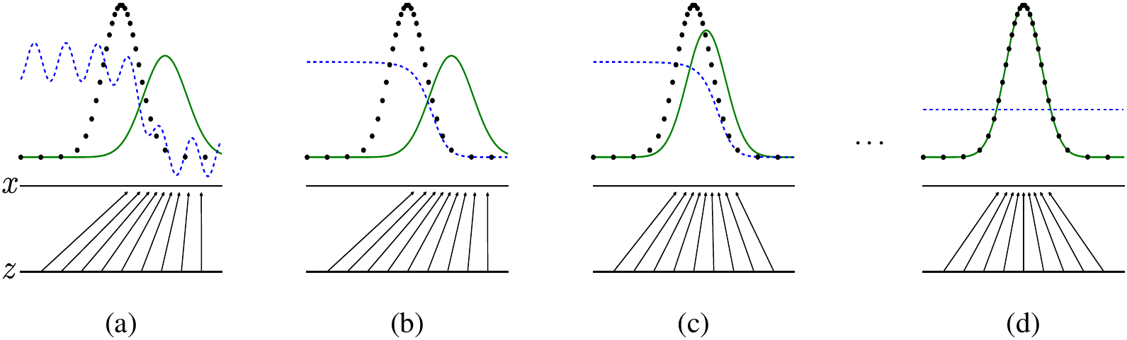
在下一节中,我们将给出对抗网络的理论分析,其本质是说明:当赋予和足够的容量时,即在非参数极限下,该训练准则能够恢复数据生成分布。关于该方法一种不那么正式、更具教学性的解释,请参见图 1。在实践中,我们必须采用迭代的数值方法来实现这一博弈。在训练的内层循环中将优化至完成在计算上代价过高,而且在有限数据集上会导致过拟合。相反,我们交替执行步对的优化和一步对的优化。只要变化得足够缓慢,这就能使始终维持在其最优解附近。这一策略类似于SML/PCD [31, 29]训练中的做法,即从一个学习步骤到下一个学习步骤持续维护来自马尔可夫链的样本,从而避免在学习的内层循环中对马尔可夫链进行预热。该过程在算法 1中进行了正式描述。
In the next section, we present a theoretical analysis of adversarial nets, essentially showing that the training criterion allows one to recover the data generating distribution as and are given enough capacity, i.e., in the non-parametric limit. See Figure 1 for a less formal, more pedagogical explanation of the approach. In practice, we must implement the game using an iterative, numerical approach. Optimizing to completion in the inner loop of training is computationally prohibitive, and on finite datasets would result in overfitting. Instead, we alternate between steps of optimizing and one step of optimizing . This results in being maintained near its optimal solution, so long as changes slowly enough. This strategy is analogous to the way that SML/PCD [31, 29] training maintains samples from a Markov chain from one learning step to the next in order to avoid burning in a Markov chain as part of the inner loop of learning. The procedure is formally presented in Algorithm 1.
在实践中,公式 1可能无法为提供足够的梯度以实现良好学习。在学习初期,当表现较差时,能够以很高的置信度拒绝样本,因为它们与训练数据明显不同。在这种情况下,会饱和。与其训练去最小化,我们可以训练去最大化。这一目标函数会产生与和动力学相同的不动点,但在学习初期能够提供强得多的梯度。
In practice, equation 1 may not provide sufficient gradient for to learn well. Early in learning, when is poor, can reject samples with high confidence because they are clearly different from the training data. In this case, saturates. Rather than training to minimize we can train to maximize . This objective function results in the same fixed point of the dynamics of and but provides much stronger gradients early in learning.
4 理论结果
4 Theoretical Results
生成器将当时得到的样本的分布隐式定义为概率分布。因此,如果给定足够的容量和训练时间,我们希望算法1能够收敛到的一个良好估计器。本节的结果是在非参数设定下得到的,例如,我们通过研究概率密度函数空间中的收敛性来表示具有无限容量的模型。
The generator implicitly defines a probability distribution as the distribution of the samples obtained when . Therefore, we would like Algorithm 1 to converge to a good estimator of , if given enough capacity and training time. The results of this section are done in a non-parametric setting, e.g. we represent a model with infinite capacity by studying convergence in the space of probability density functions.
我们将在4.1节中证明,当时,该极小极大博弈具有全局最优解。随后我们将在4.2节中证明算法1优化式1,从而得到期望的结果。
We will show in section 4.1 that this minimax game has a global optimum for . We will then show in section 4.2 that Algorithm 1 optimizes Eq 1, thus obtaining the desired result.
算法 1 生成对抗网络的小批量随机梯度下降训练。应用于判别器的步数是一个超参数。在我们的实验中使用了,这是代价最低的选择。
Algorithm 1 Minibatch stochastic gradient descent training of generative adversarial nets. The number of steps to apply to the discriminator, , is a hyperparameter. We used , the least expensive option in our experiments.
for 训练迭代次数 do
for number of training iterations do
for 步 do
for steps do
- 从噪声先验中采样包含个噪声样本的小批量。
- 从数据生成分布中采样包含个样本的小批量。
- 通过沿其随机梯度上升来更新判别器:
- Sample minibatch of noise samples from noise prior .
- Sample minibatch of examples from data generating distribution .
- Update the discriminator by ascending its stochastic gradient:
end for
end for
- 从噪声先验中采样包含个噪声样本的小批量。
- 通过沿其随机梯度下降来更新生成器:
- Sample minibatch of noise samples from noise prior .
- Update the generator by descending its stochastic gradient:
end for
end for
基于梯度的更新可以使用任何标准的基于梯度的学习规则。在我们的实验中使用了动量法。
The gradient-based updates can use any standard gradient-based learning rule. We used momentum in our experiments.
4.1 的全局最优性
4.1 Global Optimality of
我们首先考虑任意给定生成器对应的最优判别器。
We first consider the optimal discriminator for any given generator .
命题 1. 对于固定的,最优判别器为
Proposition 1. For fixed, the optimal discriminator is
证明。 给定任意生成器G,判别器D的训练准则是最大化量
Proof. The training criterion for the discriminator D, given any generator G, is to maximize the quantity
对于任意,函数在区间上的最大值于处取得。判别器无需在之外定义,证明完成。
For any , the function achieves its maximum in at . The discriminator does not need to be defined outside of , concluding the proof.
注意,的训练目标可以解释为最大化用于估计条件概率的对数似然,其中表示是来自(此时)还是来自(此时)。式1中的极小极大博弈现在可以重写为:
Note that the training objective for can be interpreted as maximizing the log-likelihood for estimating the conditional probability , where indicates whether comes from (with ) or from (with ). The minimax game in Eq. 1 can now be reformulated as:
定理 1. 虚拟训练准则的全局最小值当且仅当时达到。此时,取得值。
Theorem 1. The global minimum of the virtual training criterion is achieved if and only if . At that point, achieves the value .
证明。 当时,(见式2)。因此,考察时的式4,可得。为了说明这是所能达到的最佳值,并且仅在时达到,注意到
Proof. For , , (consider Eq. 2). Hence, by inspecting Eq. 4 at , we find . To see that this is the best possible value of , reached only for , observe that
并且从中减去该表达式,我们得到:
and that by subtracting this expression from , we obtain:
其中 KL 是 Kullback–Leibler 散度。我们可以在前面的表达式中识别出模型分布与数据生成过程之间的 Jensen–Shannon 散度:
where KL is the Kullback–Leibler divergence. We recognize in the previous expression the Jensen–Shannon divergence between the model’s distribution and the data generating process:
由于两个分布之间的 Jensen–Shannon 散度总是非负的,并且仅当它们相等时才为零,我们已经证明是的全局最小值,并且唯一解为,即生成模型完美复制了数据生成过程。
Since the Jensen–Shannon divergence between two distributions is always non-negative and zero only when they are equal, we have shown that is the global minimum of and that the only solution is , i.e., the generative model perfectly replicating the data generating process.
4.2 算法 1 的收敛性
4.2 Convergence of Algorithm 1
命题 2. 如果和具有足够的容量,并且在算法 1 的每一步中,判别器在给定的条件下都被允许达到其最优值,同时更新以改进准则
Proposition 2. If and have enough capacity, and at each step of Algorithm 1, the discriminator is allowed to reach its optimum given , and is updated so as to improve the criterion
则收敛到
then converges to
证明。按照上述准则中的做法,将视为的函数。注意,关于是凸的。凸函数上确界的次导数包含达到最大值点处该函数的导数。换言之,如果,并且对每个都有关于凸,那么当时,。这等价于在对应给定时的最优处,对计算一次梯度下降更新。根据定理 1 已证明的结果,关于是凸的,并且具有唯一的全局最优解,因此当的更新足够小时,收敛到,从而完成证明。
Proof. Consider as a function of as done in the above criterion. Note that is convex in . The subderivatives of a supremum of convex functions include the derivative of the function at the point where the maximum is attained. In other words, if and is convex in for every , then if . This is equivalent to computing a gradient descent update for at the optimal given the corresponding . is convex in with a unique global optima as proven in Thm 1, therefore with sufficiently small updates of , converges to , concluding the proof.
在实践中,对抗网络通过函数表示分布的一个受限族,而我们优化的是而非本身。使用多层感知机来定义会在参数空间中引入多个临界点。然而,多层感知机在实践中的优异性能表明,尽管缺乏理论保证,它们仍然是合理可用的模型。
In practice, adversarial nets represent a limited family of distributions via the function , and we optimize rather than itself. Using a multilayer perceptron to define introduces multiple critical points in parameter space. However, the excellent performance of multilayer perceptrons in practice suggests that they are a reasonable model to use despite their lack of theoretical guarantees.
5 实验
5 Experiments
我们在多个数据集上训练了对抗网络,包括MNIST[23]、Toronto Face Database(TFD)[28]以及CIFAR-10 [21]。生成器网络使用了整流线性激活函数[19, 9]与sigmoid激活函数的混合,而判别器网络使用了maxout [10]激活函数。在训练判别器网络时应用了Dropout [17]。尽管我们的理论框架允许在生成器的中间层使用dropout及其他噪声,但我们仅将噪声作为生成器网络最底层的输入。
We trained adversarial nets on a range of datasets including MNIST[23], the Toronto Face Database (TFD) [28], and CIFAR-10 [21]. The generator nets used a mixture of rectifier linear activations [19, 9] and sigmoid activations, while the discriminator net used maxout [10] activations. Dropout [17] was applied in training the discriminator net. While our theoretical framework permits the use of dropout and other noise at intermediate layers of the generator, we used noise as the input to only the bottommost layer of the generator network.
我们通过对由生成的样本拟合高斯Parzen窗,并报告该分布下的对数似然,来估计测试集数据在下的概率。参数
We estimate probability of the test set data under by fitting a Gaussian Parzen window to the samples generated with and reporting the log-likelihood under this distribution. The parameter
表 1:基于Parzen窗的对数似然估计。MNIST上的报告数值是测试集样本对数似然的均值,均值标准误差在样本间计算得到。在TFD上,我们在数据集各折之间计算标准误差,并使用每一折的验证集选择不同的。在TFD上,在每一折上通过交叉验证确定,并计算每一折上的平均对数似然。对于MNIST,我们与该数据集实值版本(而非二值版本)的其他模型进行比较。
Table 1: Parzen window-based log-likelihood estimates. The reported numbers on MNIST are the mean log-likelihood of samples on test set, with the standard error of the mean computed across examples. On TFD, we computed the standard error across folds of the dataset, with a different chosen using the validation set of each fold. On TFD, was cross validated on each fold and mean log-likelihood on each fold were computed. For MNIST we compare against other models of the real-valued (rather than binary) version of dataset.
这些高斯分布的参数通过在验证集上进行交叉验证得到。该过程由Breuleux et al. [8]提出,并用于多种无法计算精确似然的生成模型[25, 3, 5]。结果见表 1。这种似然估计方法具有较高方差,在高维空间中表现不佳,但据我们所知,它是当前可用的最佳方法。那些能够采样却无法直接估计似然的生成模型的发展,促使人们进一步研究如何评估此类模型。
of the Gaussians was obtained by cross validation on the validation set. This procedure was introduced in Breuleux et al. [8] and used for various generative models for which the exact likelihood is not tractable [25, 3, 5]. Results are reported in Table 1. This method of estimating the likelihood has somewhat high variance and does not perform well in high dimensional spaces but it is the best method available to our knowledge. Advances in generative models that can sample but not estimate likelihood directly motivate further research on how to evaluate such models.
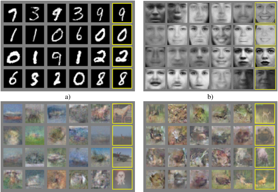
在图 2和图 3中,我们展示了训练后从生成器网络中抽取的样本。尽管我们并不声称这些样本优于现有方法生成的样本,但我们认为这些样本至少能够与文献中较好的生成模型相竞争,并体现了对抗框架的潜力。
In Figures 2 and 3 we show samples drawn from the generator net after training. While we make no claim that these samples are better than samples generated by existing methods, we believe that these samples are at least competitive with the better generative models in the literature and highlight the potential of the adversarial framework.

| 深度有向图模型 | 深度无向图模型 | 生成式自编码器 | 对抗模型 | |
|---|---|---|---|---|
| 训练 | 训练期间需要推理。 | 训练期间需要推理。需要MCMC来近似配分函数梯度。 | 在混合能力与重构生成能力之间强制权衡 | 使判别器与生成器同步。Helvetica。 |
| 推理 | 学习得到的近似推理 | 变分推理 | 基于MCMC的推理 | 学习得到的近似推理 |
| 采样 | 无困难 | 需要马尔可夫链 | 需要马尔可夫链 | 无困难 |
| 评估 | 不可处理,可用AIS近似 | 不可处理,可用AIS近似 | 未显式表示,可用Parzen密度估计近似 | 未显式表示,可用Parzen密度估计近似 |
| 模型设计 | 几乎所有模型都会遇到极大困难 | 需要精心设计以保证多种性质 | 理论上允许任意可微函数 | 理论上允许任意可微函数 |
| Deep directed graphical models | Deep undirected graphical models | Generative autoencoders | Adversarial models | |
|---|---|---|---|---|
| Training | Inference needed during training. | Inference needed during training. MCMC needed to approximate partition function gradient. | Enforced tradeoff between mixing and power of reconstruction generation | Synchronizing the discriminator with the generator. Helvetica. |
| Inference | Learned approximate inference | Variational inference | MCMC-based inference | Learned approximate inference |
| Sampling | No difficulties | Requires Markov chain | Requires Markov chain | No difficulties |
| Evaluating | Intractable, may be approximated with AIS | Intractable, may be approximated with AIS | Not explicitly represented, may be approximated with Parzen density estimation | Not explicitly represented, may be approximated with Parzen density estimation |
| Model design | Nearly all models incur extreme difficulty | Careful design needed to ensure multiple properties | Any differentiable function is theoretically permitted | Any differentiable function is theoretically permitted |
表 2:生成建模中的挑战:对深度生成建模不同方法在涉及模型的各项主要操作中所遇到困难的总结。
Table 2: Challenges in generative modeling: a summary of the difficulties encountered by different approaches to deep generative modeling for each of the major operations involving a model.
6 优势与劣势
6 Advantages and disadvantages
与先前的建模框架相比,这一新框架既有优势也有劣势。其劣势主要在于不存在对的显式表示,并且在训练过程中必须与保持良好同步(特别是,为了避免“Helvetica 情形”,即将过多的取值坍缩到同一个取值,从而缺乏足够的多样性来建模,在不更新的情况下不能对进行过多训练);这一点类似于玻尔兹曼机的负链必须在学习步骤之间保持最新状态。其优势在于永远不需要马尔可夫链,只需使用反向传播来获得梯度,学习过程中不需要推理,并且可以将各种各样的函数纳入模型。表 2总结了生成对抗网络与其他生成建模方法的比较。
This new framework comes with advantages and disadvantages relative to previous modeling frameworks. The disadvantages are primarily that there is no explicit representation of , and that must be synchronized well with during training (in particular, must not be trained too much without updating , in order to avoid “the Helvetica scenario” in which collapses too many values of to the same value of to have enough diversity to model ), much as the negative chains of a Boltzmann machine must be kept up to date between learning steps. The advantages are that Markov chains are never needed, only backprop is used to obtain gradients, no inference is needed during learning, and a wide variety of functions can be incorporated into the model. Table 2 summarizes the comparison of generative adversarial nets with other generative modeling approaches.
上述优势主要体现在计算方面。由于生成器网络并非直接利用数据样例进行更新,而仅通过流经判别器的梯度进行更新,对抗模型还可能因此获得某些统计上的优势。这意味着输入的各个组成部分不会被直接复制到生成器的参数中。对抗网络的另一个优势是,它们能够表示非常尖锐甚至退化的分布;而基于马尔可夫链的方法则要求分布具有一定程度的模糊性,以便链能够在不同模态之间实现混合。
The aforementioned advantages are primarily computational. Adversarial models may also gain some statistical advantage from the generator network not being updated directly with data examples, but only with gradients flowing through the discriminator. This means that components of the input are not copied directly into the generator’s parameters. Another advantage of adversarial networks is that they can represent very sharp, even degenerate distributions, while methods based on Markov chains require that the distribution be somewhat blurry in order for the chains to be able to mix between modes.
7 结论与未来工作
7 Conclusions and future work
该框架允许许多直接的扩展:
This framework admits many straightforward extensions:
- 通过将作为输入同时加入和,可以得到一个条件生成模型。
- 通过训练一个辅助网络来根据预测,可以实现学习得到的近似推理。这与由wake-sleep算法[15]训练的推理网络类似,但其优点在于,在生成器网络完成训练之后,可以针对一个固定的生成器网络来训练推理网络。
- A conditional generative model can be obtained by adding as input to both and .
- Learned approximate inference can be performed by training an auxiliary network to predict given . This is similar to the inference net trained by the wake-sleep algorithm [15] but with the advantage that the inference net may be trained for a fixed generator net after the generator net has finished training.
- 通过训练一族共享参数的条件模型,可以近似地对所有条件分布进行建模,其中是的索引集合的一个子集。从本质上讲,可以利用对抗网络来实现确定性MP-DBM [11]的随机扩展。
- 半监督学习:来自判别器或推理网络的特征,能够在可用标注数据有限时提高分类器的性能。
- 效率改进:通过设计更好的方法来协调和,或者在训练期间确定更优的采样分布,可以大幅加速训练。
- One can approximately model all conditionals where is a subset of the indices of by training a family of conditional models that share parameters. Essentially, one can use adversarial nets to implement a stochastic extension of the deterministic MP-DBM [11].
- Semi-supervised learning: features from the discriminator or inference net could improve performance of classifiers when limited labeled data is available.
- Efficiency improvements: training could be accelerated greatly by divising better methods for coordinating and or determining better distributions to sample from during training.
本文已经证明了对抗建模框架的可行性,表明这些研究方向可能是有价值的。
This paper has demonstrated the viability of the adversarial modeling framework, suggesting that these research directions could prove useful.
致谢
Acknowledgments
我们感谢Patrice Marcotte、Olivier Delalleau、Kyunghyun Cho、Guillaume Alain和Jason Yosinski所进行的富有帮助的讨论。Yann Dauphin与我们分享了他的Parzen窗评估代码。我们感谢Pylearn2 [12]和Theano [7, 1]的开发者,尤其是Frédéric Bastien,他分享了一项专门为本项目提供帮助的Theano特性。Arnaud Bergeron在排版方面提供了极其重要的支持。我们还感谢CIFAR和Canada Research Chairs提供资金支持,并感谢Compute Canada和Calcul Québec提供计算资源。Ian Goodfellow获得了2013年Google深度学习奖学金的资助。最后,我们感谢Les Trois Brasseurs激发了我们的创造力。
We would like to acknowledge Patrice Marcotte, Olivier Delalleau, Kyunghyun Cho, Guillaume Alain and Jason Yosinski for helpful discussions. Yann Dauphin shared his Parzen window evaluation code with us. We would like to thank the developers of Pylearn2 [12] and Theano [7, 1], particularly Frédéric Bastien who shared a Theano feature specifically to benefit this project. Arnaud Bergeron provided much-needed support with typesetting. We would also like to thank CIFAR, and Canada Research Chairs for funding, and Compute Canada, and Calcul Québec for providing computational resources. Ian Goodfellow is supported by the 2013 Google Fellowship in Deep Learning. Finally, we would like to thank Les Trois Brasseurs for stimulating our creativity.
Notes
- Jean Pouget-Abadie从Ecole Polytechnique访问蒙特利尔大学。
- Sherjil Ozair从Indian Institute of Technology Delhi访问蒙特利尔大学
- Yoshua Bengio是CIFAR高级研究员。
- 所有代码和超参数可在http://www.github.com/goodfeli/adversarial获得
References
- Bastien, F., Lamblin, P., Pascanu, R., Bergstra, J., Goodfellow, I. J., Bergeron, A., Bouchard, N., and Bengio, Y. (2012). Theano: new features and speed improvements. Deep Learning and Unsupervised Feature Learning NIPS 2012 Workshop.
- Bengio, Y. (2009). *Learning deep architectures for AI.* Now Publishers.
- Bengio, Y., Mesnil, G., Dauphin, Y., and Rifai, S. (2013a). Better mixing via deep representations. In *ICML’13*.
- Bengio, Y., Yao, L., Alain, G., and Vincent, P. (2013b). Generalized denoising auto-encoders as generative models. In *NIPS26*. Nips Foundation.
- Bengio, Y., Thibodeau-Laufer, E., and Yosinski, J. (2014a). Deep generative stochastic networks trainable by backprop. In *ICML’14*.
- Bengio, Y., Thibodeau-Laufer, E., Alain, G., and Yosinski, J. (2014b). Deep generative stochastic networks trainable by backprop. In *Proceedings of the 30th International Conference on Machine Learning (ICML’14)*.
- Bergstra, J., Breuleux, O., Bastien, F., Lamblin, P., Pascanu, R., Desjardins, G., Turian, J., Warde-Farley, D., and Bengio, Y. (2010). Theano: a CPU and GPU math expression compiler. In *Proceedings of the Python for Scientific Computing Conference (SciPy)*. Oral Presentation.
- Breuleux, O., Bengio, Y., and Vincent, P. (2011). Quickly generating representative samples from an RBM-derived process. *Neural Computation*, **23**(8), 2053–2073.
- Glorot, X., Bordes, A., and Bengio, Y. (2011). Deep sparse rectifier neural networks. In *AISTATS’2011*.
- Goodfellow, I. J., Warde-Farley, D., Mirza, M., Courville, A., and Bengio, Y. (2013a). Maxout networks. In *ICML’2013*.
- Goodfellow, I. J., Mirza, M., Courville, A., and Bengio, Y. (2013b). Multi-prediction deep Boltzmann machines. In *NIPS’2013*.
- Goodfellow, I. J., Warde-Farley, D., Lamblin, P., Dumoulin, V., Mirza, M., Pascanu, R., Bergstra, J., Bastien, F., and Bengio, Y. (2013c). Pylearn2: a machine learning research library. *arXiv preprint arXiv:1308.4214*.
- Gutmann, M. and Hyvarinen, A. (2010). Noise-contrastive estimation: A new estimation principle for unnormalized statistical models. In *AISTATS’2010*.
- Hinton, G., Deng, L., Dahl, G. E., Mohamed, A., Jaitly, N., Senior, A., Vanhoucke, V., Nguyen, P., Sainath, T., and Kingsbury, B. (2012a). Deep neural networks for acoustic modeling in speech recognition. *IEEE Signal Processing Magazine*, **29**(6), 82–97.
- Hinton, G. E., Dayan, P., Frey, B. J., and Neal, R. M. (1995). The wake-sleep algorithm for unsupervised neural networks. *Science*, **268**, 1558–1161.
- Hinton, G. E., Osindero, S., and Teh, Y. (2006). A fast learning algorithm for deep belief nets. *Neural Computation*, **18**, 1527–1554.
- Hinton, G. E., Srivastava, N., Krizhevsky, A., Sutskever, I., and Salakhutdinov, R. (2012b). Improving neural networks by preventing co-adaptation of feature detectors. Technical report, arXiv:1207.0580.
- Hyvärinen, A. (2005). Estimation of non-normalized statistical models using score matching. *J. Machine Learning Res.*, **6**.
- Jarrett, K., Kavukcuoglu, K., Ranzato, M., and LeCun, Y. (2009). What is the best multi-stage architecture for object recognition? In *Proc. International Conference on Computer Vision (ICCV’09)*, pages 2146–2153. IEEE.
- Kingma, D. P. and Welling, M. (2014). Auto-encoding variational bayes. In *Proceedings of the International Conference on Learning Representations (ICLR)*.
- Krizhevsky, A. and Hinton, G. (2009). Learning multiple layers of features from tiny images. Technical report, University of Toronto.
- Krizhevsky, A., Sutskever, I., and Hinton, G. (2012). ImageNet classification with deep convolutional neural networks. In *NIPS’2012*. Read it here
- LeCun, Y., Bottou, L., Bengio, Y., and Haffner, P. (1998). Gradient-based learning applied to document recognition. *Proceedings of the IEEE*, **86**(11), 2278–2324. Read it here
- Rezende, D. J., Mohamed, S., and Wierstra, D. (2014). Stochastic backpropagation and approximate inference in deep generative models. Technical report, arXiv:1401.4082.
- Rifai, S., Bengio, Y., Dauphin, Y., and Vincent, P. (2012). A generative process for sampling contractive auto-encoders. In *ICML’12*.
- Salakhutdinov, R. and Hinton, G. E. (2009). Deep Boltzmann machines. In *AISTATS’2009*, pages 448–455.
- Smolensky, P. (1986). Information processing in dynamical systems: Foundations of harmony theory. In D. E. Rumelhart and J. L. McClelland, editors, *Parallel Distributed Processing*, volume 1, chapter 6, pages 194–281. MIT Press, Cambridge.
- Susskind, J., Anderson, A., and Hinton, G. E. (2010). The Toronto face dataset. Technical Report UTML TR 2010-001, U. Toronto.
- Tieleman, T. (2008). Training restricted Boltzmann machines using approximations to the likelihood gradient. In W. W. Cohen, A. McCallum, and S. T. Roweis, editors, *ICML 2008*, pages 1064–1071. ACM.
- Vincent, P., Larochelle, H., Bengio, Y., and Manzagol, P.-A. (2008). Extracting and composing robust features with denoising autoencoders. In *ICML 2008*.
- Younes, L. (1999). On the convergence of Markovian stochastic algorithms with rapidly decreasing ergodicity rates. *Stochastics and Stochastic Reports*, **65**(3), 177–228.
Read off the page by a vision model reading the page images using gpt-6-astra. Translated into 中文 by gpt-5, against glossary version 5. Translated from the English.
Read off the page by a vision model reading the page images using gpt-6-astra.